Chapter 7: Confidence Intervals

Chapter 7 Homework
7.1 homework.
Among various ethnic groups, the standard deviation of heights is known to be approximately three inches. We wish to construct a 95% confidence interval for the mean height of male Swedes. Forty-eight male Swedes are surveyed. The sample mean is 71 inches. The sample standard deviation is 2.8 inches.
Construct a 95% confidence interval for the population mean height of male Swedes.

Announcements for 84 upcoming engineering conferences were randomly picked from a stack of IEEE Spectrum magazines. The mean length of the conferences was 3.94 days, with a standard deviation of 1.28 days. Assume the underlying population is normal.
- In words, define the random variables X and [latex]\overline{X}[/latex].
- Which distribution should you use for this problem? Explain your choice.
- State the confidence interval.
- Sketch the graph.
- Calculate the error bound.
Suppose that an accounting firm does a study to determine the time needed to complete one person’s tax forms. It randomly surveys 100 people. The sample mean is 23.6 hours. There is a known standard deviation of 7.0 hours. The population distribution is assumed to be normal.
- [latex]\overline{x}[/latex] =________
- σ =________
- n =________
- If the firm wished to increase its level of confidence and keep the error bound the same by taking another survey, what changes should it make?
- If the firm did another survey, kept the error bound the same, and only surveyed 49 people, what would happen to the level of confidence? Why?
- Suppose that the firm decided that it needed to be at least 96% confident of the population mean length of time to within one hour. How would the number of people the firm surveys change? Why?
- [latex]\overline{x}[/latex] = 23.6
- [latex]\sigma[/latex] = 7
- X is the time needed to complete an individual tax form. [latex]\overline{X}[/latex] is the mean time to complete tax forms from a sample of 100 customers.
- (22.228, 24.972)
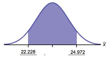
- EBM = 1.372
- It will need to change the sample size. The firm needs to determine what the confidence level should be, then apply the error bound formula to determine the necessary sample size.
- The confidence level would increase as a result of a larger interval. Smaller sample sizes result in more variability. To capture the true population mean, we need to have a larger interval.
- According to the error bound formula, the firm needs to survey 206 people. Since we increase the confidence level, we need to increase either our error bound or the sample size.
A sample of 16 small bags of the same brand of candies was selected. Assume that the population distribution of bag weights is normal. The weight of each bag was then recorded. The mean weight was two ounces with a standard deviation of 0.12 ounces. The population standard deviation is known to be 0.1 ounce.
- s x =________
- In words, define the random variable X .
- In words, define the random variable [latex]\overline{X}[/latex].
- In complete sentences, explain why the confidence interval in part f is larger than the confidence interval in part e.
- In complete sentences, give an interpretation of what the interval in part f means.
A camp director is interested in the mean number of letters each child sends during his or her camp session. The population standard deviation is known to be 2.5. A survey of 20 campers is taken. The mean from the sample is 7.9 with a sample standard deviation of 2.8.
- Define the random variables X and [latex]\overline{X}[/latex] in words.
- What will happen to the error bound and confidence interval if 500 campers are surveyed? Why?
N [latex]7.9\left(\frac{2.5}{\sqrt{20}}\right)[/latex]
What is meant by the term “90% confident” when constructing a confidence interval for a mean?
- If we took repeated samples, approximately 90% of the samples would produce the same confidence interval.
- If we took repeated samples, approximately 90% of the confidence intervals calculated from those samples would contain the sample mean.
- If we took repeated samples, approximately 90% of the confidence intervals calculated from those samples would contain the true value of the population mean.
- If we took repeated samples, the sample mean would equal the population mean in approximately 90% of the samples.
The Federal Election Commission collects information about campaign contributions and disbursements for candidates and political committees each election cycle. During the 2012 campaign season, there were 1,619 candidates for the House of Representatives across the United States who received contributions from individuals. [link] shows the total receipts from individuals for a random selection of 40 House candidates rounded to the nearest 💲100. The standard deviation for this data to the nearest hundred is σ = 💲909,200.
| 💲3,600 | 💲1,243,900 | 💲10,900 | 💲385,200 | 💲581,500 |
| 💲7,400 | 💲2,900 | 💲400 | 💲3,714,500 | 💲632,500 |
| 💲391,000 | 💲467,400 | 💲56,800 | 💲5,800 | 💲405,200 |
| 💲733,200 | 💲8,000 | 💲468,700 | 💲75,200 | 💲41,000 |
| 💲13,300 | 💲9,500 | 💲953,800 | 💲1,113,500 | 💲1,109,300 |
| 💲353,900 | 💲986,100 | 💲88,600 | 💲378,200 | 💲13,200 |
| 💲3,800 | 💲745,100 | 💲5,800 | 💲3,072,100 | 💲1,626,700 |
| 💲512,900 | 💲2,309,200 | 💲6,600 | 💲202,400 | 💲15,800 |
- Find the point estimate for the population mean.
- Using 95% confidence, calculate the error bound.
- Create a 95% confidence interval for the mean total individual contributions.
- Interpret the confidence interval in the context of the problem.
- [latex]\overline{x}[/latex] = 💲568,873
EBM = [latex]{z}_{0.025}\frac{\sigma }{\sqrt{n}}[/latex] = 1.96 [latex]\frac{909200}{\sqrt{40}}[/latex] = 💲281,764
[latex]\overline{x}[/latex] + EBM = 568,873 + 281,764 = 850,637
Alternate solution:
Press STAT and arrow over to TESTS .
- Arrow down to 7:ZInterval .
Press ENTER .
- Arrow to Stats and press ENTER .
- σ : 909,200
- [latex]\overline{x}[/latex]: 568,873
- Arrow down to Calculate and press ENTER .
- The confidence interval is (💲287,114, 💲850,632).
- Notice the small difference between the two solutions—these differences are simply due to rounding errors in the hand calculations.
- We estimate with 95% confidence that the mean amount of contributions received from all individuals by House candidates is between 💲287,109 and 💲850,637.
The American Community Survey (ACS), part of the United States Census Bureau, conducts a yearly census similar to the one taken every ten years, but with a smaller percentage of participants. The most recent survey estimates with 90% confidence that the mean household income in the U.S. falls between 💲69,720 and 💲69,922. Find the point estimate for mean U.S. household income and the error bound for mean U.S. household income.
The average height of young adult males has a normal distribution with standard deviation of 2.5 inches. You want to estimate the mean height of students at your college or university to within one inch with 93% confidence. How many male students must you measure?
Use the formula for EBM , solved for n :
[latex]n=\frac{{z}^{2}{\sigma}^{2}}{EB{M}^{2}}[/latex]
From the statement of the problem, you know that σ = 2.5, and you need EBM = 1.
z = z 0.035 = 1.812
(This is the value of z for which the area under the density curve to the right of z is 0.035.)
[latex]n=\frac{{z}^{2}{\sigma}^{2}}{EB{M}^{2}}=\frac{{1.812}^{2}{2.5}^{2}}{{1}^{2}}\approx 20.52[/latex]
You need to measure at least 21 male students to achieve your goal.
7.2 Homework
In six packages of “The Flintstones® Real Fruit Snacks” there were five Bam-Bam snack pieces. The total number of snack pieces in the six bags was 68. We wish to calculate a 96% confidence interval for the population proportion of Bam-Bam snack pieces.
- Define the random variables X and P ′ in words.
- Which distribution should you use for this problem? Explain your choice
- Calculate p ′.
- Do you think that six packages of fruit snacks yield enough data to give accurate results? Why or why not?
A random survey of enrollment at 35 community colleges across the United States yielded the following figures: 6,414; 1,550; 2,109; 9,350; 21,828; 4,300; 5,944; 5,722; 2,825; 2,044; 5,481; 5,200; 5,853; 2,750; 10,012; 6,357; 27,000; 9,414; 7,681; 3,200; 17,500; 9,200; 7,380; 18,314; 6,557; 13,713; 17,768; 7,493; 2,771; 2,861; 1,263; 7,285; 28,165; 5,080; 11,622. Assume the underlying population is normal.
Construct a 95% confidence interval for the population mean enrollment at community colleges in the United States.
- CI: (6244, 11,014)

- It will become smaller
Suppose that a committee is studying whether or not there is waste of time in our judicial system. It is interested in the mean amount of time individuals waste at the courthouse waiting to be called for jury duty. The committee randomly surveyed 81 people who recently served as jurors. The sample mean wait time was eight hours with a sample standard deviation of four hours.
- [latex]\overline{x}[/latex] = __________
- [latex]{s}_{x}[/latex] = __________
- n = __________
- n – 1 = __________
- Define the random variables [latex]X[/latex] and [latex]\overline{X}[/latex] in words.
- Explain in a complete sentence what the confidence interval means.
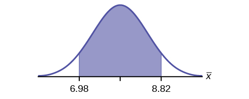
A pharmaceutical company makes tranquilizers. It is assumed that the distribution for the length of time they last is approximately normal. Researchers in a hospital used the drug on a random sample of nine patients. The effective period of the tranquilizer for each patient (in hours) was as follows: 2.7; 2.8; 3.0; 2.3; 2.3; 2.2; 2.8; 2.1; and 2.4.
- Define the random variable [latex]X[/latex] in words.
- Define the random variable [latex]\overline{X}[/latex] in words.
- What does it mean to be “95% confident” in this problem?
- [latex]\overline{x}[/latex] = 2.51
- [latex]{s}_{x}[/latex] = 0.318
- the effective length of time for a tranquilizer
- the mean effective length of time of tranquilizers from a sample of nine patients
- CI: (2.27, 2.76)
- Check student’s solution.
- If we were to sample many groups of nine patients, 95% of the samples would contain the true population mean length of time.
Suppose that 14 children, who were learning to ride two-wheel bikes, were surveyed to determine how long they had to use training wheels. It was revealed that they used them an average of six months with a sample standard deviation of three months. Assume that the underlying population distribution is normal.
- Define the random variable[latex]\overline{X}[/latex] in words.
- Why would the error bound change if the confidence level were lowered to 90%?
The Federal Election Commission (FEC) collects information about campaign contributions and disbursements for candidates and political committees each election cycle. A political action committee (PAC) is a committee formed to raise money for candidates and campaigns. A Leadership PAC is a PAC formed by a federal politician (senator or representative) to raise money to help other candidates’ campaigns.
The FEC has reported financial information for 556 Leadership PACs that operated during the 2011–2012 election cycle. The following table shows the total receipts during this cycle for a random selection of 20 Leadership PACs.
| 💲46,500.00 | 💲0 | 💲40,966.50 | 💲105,887.20 | 💲5,175.00 |
| 💲29,050.00 | 💲19,500.00 | 💲181,557.20 | 💲31,500.00 | 💲149,970.80 |
| 💲2,555,363.20 | 💲12,025.00 | 💲409,000.00 | 💲60,521.70 | 💲18,000.00 |
| 💲61,810.20 | 💲76,530.80 | 💲119,459.20 | 💲0 | 💲63,520.00 |
| 💲6,500.00 | 💲502,578.00 | 💲705,061.10 | 💲708,258.90 | 💲135,810.00 |
| 💲2,000.00 | 💲2,000.00 | 💲0 | 💲1,287,933.80 | 💲219,148.30 |
[latex]\overline{x}=$251,854.23[/latex]
[latex]s=\text{ }$521,130.41[/latex]
Use this sample data to construct a 96% confidence interval for the mean amount of money raised by all Leadership PACs during the 2011–2012 election cycle. Use the Student’s t-distribution.
[latex]s=\$521,130.41[/latex]
Note that we are not given the population standard deviation, only the standard deviation of the sample.
There are 30 measures in the sample, so n = 30, and df = 30 – 1 = 29
CL = 0.96, so α = 1 – CL = 1 – 0.96 = 0.04
[latex]\frac{\alpha }{2}=0.02{t}_{\frac{\alpha }{2}}={t}_{0.02}[/latex] = 2.150
[latex]EBM=t_{\frac{\alpha}{2}}\left(\frac{s}{\sqrt{n}}\right)=2.150\left(\frac{521,130.41}{\sqrt{30}}\right)\approx \$204,561.66[/latex]
[latex]\overline{x}[/latex] – EBM = $251,854.23 – $204,561.66 = $47,292.57
[latex]\overline{x}[/latex] + EBM = $251,854.23+ $204,561.66 = $456,415.89
We estimate with 96% confidence that the mean amount of money raised by all Leadership PACs during the 2011–2012 election cycle lies between $47,292.57 and $456,415.89.
Alternate Solution
Enter the data as a list.
Arrow down to 8:TInterval .
Arrow to Data and press ENTER .
Arrow down and enter the name of the list where the data is stored.
Enter Freq : 1
Enter C-Level : 0.96
Arrow down to Calculate and press Enter .
The 96% confidence interval is ($47,262, $456,447).
The difference between solutions arises from rounding differences.
Forbes magazine published data on the best small firms in 2012. These were firms that had been publicly traded for at least a year, have a stock price of at least $5 per share, and have reported annual revenue between $5 million and $1 billion. The [link] shows the ages of the corporate CEOs for a random sample of these firms.
| 48 | 58 | 51 | 61 | 56 |
| 59 | 74 | 63 | 53 | 50 |
| 59 | 60 | 60 | 57 | 46 |
| 55 | 63 | 57 | 47 | 55 |
| 57 | 43 | 61 | 62 | 49 |
| 67 | 67 | 55 | 55 | 49 |
Use this sample data to construct a 90% confidence interval for the mean age of CEO’s for these top small firms. Use the Student's t-distribution.
Unoccupied seats on flights cause airlines to lose revenue. Suppose a large airline wants to estimate its mean number of unoccupied seats per flight over the past year. To accomplish this, the records of 225 flights are randomly selected and the number of unoccupied seats is noted for each of the sampled flights. The sample mean is 11.6 seats and the sample standard deviation is 4.1 seats.
- n -1 = __________
- Construct a 92% confidence interval for the population mean number of unoccupied seats per flight.
- [latex]\overline{x}[/latex] =
- [latex]{s}_{x}[/latex] =
- X is the number of unoccupied seats on a single flight. [latex]\overline{X}[/latex] is the mean number of unoccupied seats from a sample of 225 flights.
- CI: (11.12 , 12.08)
In a recent sample of 84 used car sales costs, the sample mean was $6,425 with a standard deviation of $3,156. Assume the underlying distribution is approximately normal.
- Explain what a “95% confidence interval” means for this study.
Six different national brands of chocolate chip cookies were randomly selected at the supermarket. The grams of fat per serving are as follows: 8; 8; 10; 7; 9; 9. Assume the underlying distribution is approximately normal.
- If you wanted a smaller error bound while keeping the same level of confidence, what should have been changed in the study before it was done?
- Go to the store and record the grams of fat per serving of six brands of chocolate chip cookies.
- Calculate the mean.
- Is the mean within the interval you calculated in part a? Did you expect it to be? Why or why not?
- CI: (7.64 , 9.36)

- The sample should have been increased.
- Answers will vary.
A survey of the mean number of cents off that coupons give was conducted by randomly surveying one coupon per page from the coupon sections of a recent San Jose Mercury News. The following data were collected: 20¢; 75¢; 50¢; 65¢; 30¢; 55¢; 40¢; 40¢; 30¢; 55¢; $1.50; 40¢; 65¢; 40¢. Assume the underlying distribution is approximately normal.
- If many random samples were taken of size 14, what percent of the confidence intervals constructed should contain the population mean worth of coupons? Explain why.
Use the following information to answer the next two exercises: A quality control specialist for a restaurant chain takes a random sample of size 12 to check the amount of soda served in the 16 oz. serving size. The sample mean is 13.30 with a sample standard deviation of 1.55. Assume the underlying population is normally distributed.
Find the 95% Confidence Interval for the true population mean for the amount of soda served.
- (12.42, 14.18)
- (12.32, 14.29)
- (12.50, 14.10)
- Impossible to determine
What is the error bound?
7.3 Homework
Insurance companies are interested in knowing the population percentage of drivers who always buckle up before riding in a car.
- When designing a study to determine this population proportion, what is the minimum number you would need to survey to be 95% confident that the population proportion is estimated to within 0.03?
- If it were later determined that it was important to be more than 95% confident and a new survey was commissioned, how would that affect the minimum number you would need to survey? Why?
- The sample size would need to be increased since the critical value increases as the confidence level increases.
Suppose that the insurance companies did do a survey. They randomly surveyed 400 drivers and found that 320 claimed they always buckle up. We are interested in the population proportion of drivers who claim they always buckle up.
- x = __________
- p ′ = __________
- Define the random variables X and P ′, in words.
- If this survey were done by telephone, list three difficulties the companies might have in obtaining random results.
According to a recent survey of 1,200 people, 61% feel that the president is doing an acceptable job. We are interested in the population proportion of people who feel the president is doing an acceptable job.
X = the number of people who feel that the president is doing an acceptable job;
P ′ = the proportion of people in a sample who feel that the president is doing an acceptable job.
- CI: (0.59, 0.63)
- Check student’s solution
An article regarding interracial dating and marriage recently appeared in the Washington Post . Of the 1,709 randomly selected adults, 315 identified themselves as Latinos, 323 identified themselves as blacks, 254 identified themselves as Asians, and 779 identified themselves as whites. In this survey, 86% of blacks said that they would welcome a white person into their families. Among Asians, 77% would welcome a white person into their families, 71% would welcome a Latino, and 66% would welcome a black person.
- We are interested in finding the 95% confidence interval for the percent of all black adults who would welcome a white person into their families. Define the random variables X and P ′, in words.
Refer to the information in [link] .
- percent of all Asians who would welcome a white person into their families.
- percent of all Asians who would welcome a Latino into their families.
- percent of all Asians who would welcome a black person into their families.
- Even though the three-point estimates are different, do any of the confidence intervals overlap? Which?
- For any intervals that do overlap, in words, what does this imply about the significance of the differences in the true proportions?
- For any intervals that do not overlap, in words, what does this imply about the significance of the differences in the true proportions?
- (0.72, 0.82)
- (0.65, 0.76)
- (0.60, 0.72)
- Yes, the intervals (0.72, 0.82) and (0.65, 0.76) overlap, and the intervals (0.65, 0.76) and (0.60, 0.72) overlap.
- We can say that there does not appear to be a significant difference between the proportion of Asian adults who say that their families would welcome a white person into their families and the proportion of Asian adults who say that their families would welcome a Latino person into their families.
- We can say that there is a significant difference between the proportion of Asian adults who say that their families would welcome a white person into their families and the proportion of Asian adults who say that their families would welcome a black person into their families.
Stanford University conducted a study of whether running is healthy for men and women over age 50. During the first eight years of the study, 1.5% of the 451 members of the 50-Plus Fitness Association died. We are interested in the proportion of people over 50 who ran and died in the same eight-year period.
- Explain what a “97% confidence interval” means for this study.
A telephone poll of 1,000 adult Americans was reported in an issue of Time Magazine . One of the questions asked was “What is the main problem facing the country?” Twenty percent answered “crime.” We are interested in the population proportion of adult Americans who feel that crime is the main problem.
Construct a 95% confidence interval for the population proportion of adult Americans who feel that crime is the main problem.
Refer to [link] . Another question in the poll was “[How much are] you worried about the quality of education in our schools?” Sixty-three percent responded “a lot”. We are interested in the population proportion of adult Americans who are worried a lot about the quality of education in our schools.
Construct a 95% confidence interval for the population proportion of adult Americans who are worried a lot about the quality of education in our schools.
Use the following information to answer the next three exercises: According to a Field Poll, 79% of California adults (actual results are 400 out of 506 surveyed) feel that “education and our schools” is one of the top issues facing California. We wish to construct a 90% confidence interval for the true proportion of California adults who feel that education and the schools is one of the top issues facing California.
A point estimate for the true population proportion is:
A 90% confidence interval for the population proportion is _______.
- (0.761, 0.820)
- (0.125, 0.188)
- (0.755, 0.826)
- (0.130, 0.183)
The error bound is approximately _____.
Use the following information to answer the next two exercises: Five hundred and eleven (511) homes in a certain southern California community are randomly surveyed to determine if they meet minimal earthquake preparedness recommendations. One hundred seventy-three (173) of the homes surveyed met the minimum recommendations for earthquake preparedness, and 338 did not.
Find the confidence interval at the 90% Confidence Level for the true population proportion of southern California community homes meeting at least the minimum recommendations for earthquake preparedness.
- (0.2975, 0.3796)
- (0.6270, 0.6959)
- (0.3041, 0.3730)
- (0.6204, 0.7025)
The point estimate for the population proportion of homes that do not meet the minimum recommendations for earthquake preparedness is ______.
On May 23, 2013, Gallup reported that of the 1,005 people surveyed, 76% of U.S. workers believe that they will continue working past retirement age. The confidence level for this study was reported at 95% with a ±3% margin of error.
- Determine the estimated proportion from the sample.
- Determine the sample size.
- Identify CL and α .
- Calculate the error bound based on the information provided.
- Compare the error bound in part d to the margin of error reported by Gallup. Explain any differences between the values.
- Create a confidence interval for the results of this study.
- A reporter is covering the release of this study for a local news station. How should she explain the confidence interval to her audience?
A national survey of 1,000 adults was conducted on May 13, 2013 by Rasmussen Reports. It concluded with 95% confidence that 49% to 55% of Americans believe that big-time college sports programs corrupt the process of higher education.
- Find the point estimate and the error bound for this confidence interval.
- Can we (with 95% confidence) conclude that more than half of all American adults believe this?
- Use the point estimate from part a and n = 1,000 to calculate a 75% confidence interval for the proportion of American adults that believe that major college sports programs corrupt higher education.
- Can we (with 75% confidence) conclude that at least half of all American adults believe this?
- p′ = [latex]\frac{\text{(0}\text{.55 + 0}\text{.49)}}{\text{2}}[/latex] = 0.52; EBP = 0.55 – 0.52 = 0.03
- No, the confidence interval includes values less than or equal to 0.50. It is possible that less than half of the population believe this.
[latex]EBP=\left(1.150\right)\sqrt{\frac{0.52\left(0.48\right)}{1,000}}\approx 0.018[/latex]
( p ′ – EBP , p ′ + EBP ) = (0.52 – 0.018, 0.52 + 0.018) = (0.502, 0.538)
STAT TESTS A: 1-PropZinterval with x = (0.52)(1,000), n = 1,000, CL = 0.75.
Answer is (0.502, 0.538)
- Yes – this interval does not fall less than 0.50 so we can conclude that at least half of all American adults believe that major sports programs corrupt education – but we do so with only 75% confidence.
Public Policy Polling recently conducted a survey asking adults across the U.S. about music preferences. When asked, 80 of the 571 participants admitted that they have illegally downloaded music.
- Create a 99% confidence interval for the true proportion of American adults who have illegally downloaded music.
- This survey was conducted through automated telephone interviews on May 6 and 7, 2013. The error bound of the survey compensates for sampling error, or natural variability among samples. List some factors that could affect the survey’s outcome that are not covered by the margin of error.
- Without performing any calculations, describe how the confidence interval would change if the confidence level changed from 99% to 90%.
You plan to conduct a survey on your college campus to learn about the political awareness of students. You want to estimate the true proportion of college students on your campus who voted in the 2012 presidential election with 95% confidence and a margin of error no greater than five percent. How many students must you interview?
CL = 0.95 α = 1 – 0.95 = 0.05 [latex]\frac{\alpha }{2}[/latex] = 0.025 [latex]{z}_{\frac{\alpha }{2}}[/latex] = 1.96. Use p ′ = q ′ = 0.5.
[latex]n=\frac{{z_{\frac{\alpha}{2}}}^2 {p'} {q'}}{EBP^2}= \frac{{1.96}^2\left(0.5\right)\left(0.5\right)}{{0.05}^2}=384.16[/latex]
You need to interview at least 385 students to estimate the proportion to within 5% at 95% confidence.
In a recent Zogby International Poll, nine of 48 respondents rated the likelihood of a terrorist attack in their community as “likely” or “very likely.” Use the “plus four” method to create a 97% confidence interval for the proportion of American adults who believe that a terrorist attack in their community is likely or very likely. Explain what this confidence interval means in the context of the problem.
investigated and reported by William S. Gossett in 1908 and published under the pseudonym Student; the major characteristics of the random variable (RV) are:
It is continuous and assumes any real values. The pdf is symmetrical about its mean of zero. However, it is more spread out and flatter at the apex than the normal distribution. It approaches the standard normal distribution as n get larger. There is a "family of t–distributions: each representative of the family is completely defined by the number of degrees of freedom, which is one less than the number of data.
Introductory Statistics Copyright © 2024 by LOUIS: The Louisiana Library Network is licensed under a Creative Commons Attribution-ShareAlike 4.0 International License , except where otherwise noted.
Share This Book
Formula Review
7.1 the central limit theorem for sample means (averages).
Central limit theorem for sample means: X ¯ X ¯ ~ N ( μ x , σ x n ) ( μ x , σ x n )
Mean X ¯ X ¯ : μ x
Central limit theorem for sample means z -score and standard error of the mean: z = x ¯ − μ x ( σ x n ) z = x ¯ − μ x ( σ x n )
Standard error of the mean (standard deviation ( X ¯ X ¯ )): σ x n σ x n
7.2 The Central Limit Theorem for Sums (Optional)
Central limit theorem for sums: ∑X ~ N [( n )( μ x ),( n n )( σ x )]
Mean for sums ( ∑X ): ( n )( μ x )
Central limit theorem for sums z -score and standard deviation for sums: z for the sample mean = Σ x – ( n ) ( μ X ) ( n ) ( σ X ) z for the sample mean = Σ x – ( n ) ( μ X ) ( n ) ( σ X )
Standard deviation for sums ( ∑X ): ( n ) ( n ) ( σ x )
As an Amazon Associate we earn from qualifying purchases.
This book may not be used in the training of large language models or otherwise be ingested into large language models or generative AI offerings without OpenStax's permission.
Want to cite, share, or modify this book? This book uses the Creative Commons Attribution License and you must attribute Texas Education Agency (TEA). The original material is available at: https://www.texasgateway.org/book/tea-statistics . Changes were made to the original material, including updates to art, structure, and other content updates.
Access for free at https://openstax.org/books/statistics/pages/1-introduction
- Authors: Barbara Illowsky, Susan Dean
- Publisher/website: OpenStax
- Book title: Statistics
- Publication date: Mar 27, 2020
- Location: Houston, Texas
- Book URL: https://openstax.org/books/statistics/pages/1-introduction
- Section URL: https://openstax.org/books/statistics/pages/7-formula-review
© Jan 23, 2024 Texas Education Agency (TEA). The OpenStax name, OpenStax logo, OpenStax book covers, OpenStax CNX name, and OpenStax CNX logo are not subject to the Creative Commons license and may not be reproduced without the prior and express written consent of Rice University.
- AP Statistics Summer Assignment (Introduction to Chapter 1)
- AP Class Notes and HW Answers
- Algebra I Assignment Sheets
- Algebra 1 Notes and Review Answer Keys
- Honors Algebra I Assignment Sheets
- Honors Notes and Review Answer Keys
- Honors Algebra 1 Summer Assignment
AP Chapter 7 (TPS4e)
AP Stats Chapter 7 – Glossary of Important Definitions
Notes (PowerPoint Presentation)
- AP Stats 7.1 Sampling Distribution
- AP Stats 7.2 Sampling Proportions
- AP Stats 7.3 Sampling Means
In-Class Activities
- AP Stats 7.2 Sampling Proportion Activity (2020 KEY)
- AP Stats 7.3 Sampling Means Activity (2020 KEY)
- AP Stats Wrapup Ch6, 7.1 and 7.2 Assignments (2023-24)
- AP Stats Wrapup Ch7 and 8.0 Assignments (2024)
- AP Stats HW 7.1 to 7.3 answers (TPS4e)
Chapter Review :
- AP Stats Self Directed Chapter 7 Review
- AP Stats Chapter 7 Practice Test (TPS4e)
- AP Stats Chapter 7 Review HW answers (TPS4e)
More Review Problems AP Stats Chapter 7 Supplement (POD Study Guide)
- Search for:
Helping math teachers bring statistics to life

Chapter 7 - Day 6
Students struggled with….
Using appropriate notation for statistics and parameters of means and proportions.
Showing all required work for these probability problems. We look for very detailed work in these problems (pictures, formulas, work, and answer).
Remembering to check conditions for normality if not specifically asked to do so.
Remedies…
With every lesson, make sure to emphasize the correct symbols being used. Students will have tons of practice with these as the course goes on.
Whether its classwork or homework, have students reflecting on all the expectations we have had in normal distribution problems. Constantly holding these high expectations will have a huge payoff in inference.
Emphasize the importance of the conditions. Always refer to the picture at the top of Table A to constantly remind students that looking up a value on that table is only valid if we are on a normal distribution. If we want to use Table A and don't know the distribution is normal, we need to justify it is.
- Turnitin Guides
- Administrator hub
- Release notes and known issues
- Welcome to Turnitin Guides
Welcome to Turnitin’s new website for guidance!
In 2024, we migrated our comprehensive library of guidance from https://help.turnitin.com to this site, guides.turnitin.com. During this process we have taken the opportunity to take a holistic look at our content and how we structure our guides.
This page is here to help you orientate yourself with these changes and update your resources
What's new?
We have restructured the content to help you navigate it more efficiently.
We are consolidating numerous pages to make our individual guides more valuable as well as removing duplicated content.
For example, our Similarity Report guidance on help.turnitin is repeated in numerous places to cater for each individual integration and license type. On guides.turnitin this content will exist in a single place to allow for users of all integrations and licenses to find it easily. We have made slight modifications to these guides to help you understand which guides are pertinent to you and your institution.
Our guidance search has greatly improved
As a result of our content restructure, the search functionality for guides.turnitin has improved. Use the search bar at the top of any page to locate the guidance you’re searching for.
Dedicated student and administrator guidance hubs
Visit the Student hub area to locate student guidance. For students who access Turnitin via an LMS or VLE, check out the subsection Submitting to Turnitin .
Visiting the Administrator hub area to locate administrator guidance and release notes.
iThenticate and Crossref Similarity Check guidance is now located on a separate site
To improve the experience for our iThenticate and Crossref Similiarity Check customers we have move their help content onto a separate help site, guides.ithenticate.com . This will improve the search for all users.
We have also created an orientation page for this site to help users become acclimatised.
Some guidance is no longer grouped within the LMS umbrella
Some guidance which was previously provided under each LMS has been moved to sections that reflect those workflows’ outcomes. Use the table below as a cheatsheet to quickly locate guidance.
| Student guidance | |
| LMS guidance for administrators and instructors | |
| Similarity Report and AI Writing guidance | |
| Creating PeerMark assignments guidance | |
| Creating and managing QuickMarks, rubrics and grading PeerMark assignments guidance | |
| User profile guidance for administrators and instructors |
|
| Administrator account settings and migration help | |
| Release notes and known issues |
Articles in this section
- Turnitin release notes
- Integrations release notes
- Integrations Known issues
COMMENTS
Section 7.2 Homework. Refer to the accompanying data display that results from a sample of airport data speeds in Mbps. (13.046,22.15) a. Express the confidence interval in the format that uses the "less than" symbol. Given that the original listed data use one decimal place, round the confidence interval limits accordingly. b.
The critical value z𝛼/2 is the positive z value that is at the boundary separating an area of z𝛼/2 in the right tail of the standard normal distribution. Use a standard normal table to find the critical value, z𝛼/2 The area to the left of z𝛼/2 is 0.9. z𝛼/2 = z0.2/2. z𝛼/2 = z 0.1. z 0.1 = 1.28.
Section 1-1: Statistics Basics. Section 1-2: Simple Random Sampling. Section 1-3: Other Sampling Designs. ... Section 7-2: The Mean and Standard Deviation of the Sample Mean. Section 7-3: ... you'll learn how to solve your toughest homework problems. Our resource for Introductory Statistics includes answers to chapter exercises, as well as ...
Section 7.2 Homework. Ping Sa. Course. Elementary Statistics For Health And Social Sciences (STA 2014) 64 Documents. Students shared 64 documents in this course. University University of North Florida. Academic year: 2018/2019. Uploaded by: Anonymous Student.
AP Statistics Link to Chapter 7 Video Notes. YOUTUBE PLAYLIST CHAPTER 7. Power Points & Notes Outline ... Lesson 7.2 Powerpoint; Lesson 7.3 Powerpoint AP Notes Chapter 7 Homework. Key HW 7.1 Part A problems 1-8 ... Examples for 7-2 are below. Normal Calculations Involving P-Hat.
2.2 Histograms, Frequency Polygons, and Time Series Graphs; 2.3 Measures of the Location of the Data; 2.4 Box Plots; 2.5 Measures of the Center of the Data; 2.6 Skewness and the Mean, Median, and Mode; 2.7 Measures of the Spread of the Data; 2.8 Descriptive Statistics; Key Terms; Chapter Review; Formula Review; Practice; Homework; Bringing It ...
Solutions for MYLAB STATISTICS: ELEMENTARY STATISTICS. View Samples. Chapter. Section. Problem 1TY: In a survey of 1501 ninth to twelfth graders in the United States, 1215 said leaders today are more... Problem 2TY: Determine whether each number describes a population parameter or a sample statistic.
2.2 Histograms, Frequency Polygons, and Time Series Graphs; 2.3 Measures of the Location of the Data; 2.4 Box Plots; 2.5 Measures of the Center of the Data; 2.6 Skewness and the Mean, Median, and Mode; 2.7 Measures of the Spread of the Data; 2.8 Descriptive Statistics; Key Terms; Chapter Review; Formula Review; Practice; Homework; Bringing It ...
7.1 Homework. Among various ethnic groups, the standard deviation of heights is known to be approximately three inches. We wish to construct a 95% confidence interval for the mean height of male Swedes. Forty-eight male Swedes are surveyed. The sample mean is 71 inches. The sample standard deviation is 2.8 inches. ¯¯¯x x ¯ =________.
Chapter. CH7.2. Problem. 1P. Step-by-step solution. Step 1 of 1. A standard score, also called a z-score, measures the number of standard deviations you are away from the mean of the normal distribution. For example, a z score of 1.25 means that the underlying data value is 1.25 standard deviations above its mean. Back to top.
CH7.2. Problem. 1CYU1. Step-by-step solution. Step 1 of 3. The following information provided in the problem. Suppose 75% of young adult internet users watch online videos. An SRS of 1000 young adult internet users taken and calculates the proportion in this sample who watch online videos. Step 2 of 3.
Access Essentials of Statistics Plus MyStatLab with Pearson eText -- Access Card Package 6th Edition Chapter 7.2 solutions now. Our solutions are written by Chegg experts so you can be assured of the highest quality!
2.2 Histograms, Frequency Polygons, and Time Series Graphs; 2.3 Measures of the Location of the Data; 2.4 Box Plots; 2.5 Measures of the Center of the Data; 2.6 Skewness and the Mean, Median, and Mode; 2.7 Measures of the Spread of the Data; 2.8 Descriptive Statistics; Key Terms; Chapter Review; Formula Review; Practice; Homework; Bringing It ...
Stats 7.3. Mean and Standard Deviation of the Sampling Distribution of x̅. Click the card to flip 👆. Suppose that x̅ is the mean of an SRS of size n drawn from a large population with mean µ and standard deviation σ, then: The mean of the sampling distribution of x̅ is µ of x̅ = µ. The standard deviation of the sampling distribution ...
STAT22000 Homework 7 Solutions. All page, section, and exercise numbers below refer to the course text (OpenIntro Statistics, 4th edition, by Diez, Barr, and Cetinkaya-Rundel.). Reading: Section 7. Problems for Self-Study : (Do Not Turn In) Exercise 7, 7, 7, 7, 711 on p-261. The answers can be found at the end of the book. Problems to Turn In:
Using Statcrunch to solve problems when the "View an Example" is using XLSTAT.
AP Stats 7.2 Sampling Proportion Activity (2020 KEY) AP Stats 7.3 Sampling Means Activity (2020 KEY) HW. AP Stats Wrapup Ch6, 7.1 and 7.2 Assignments (2023-24) AP Stats Wrapup Ch7 and 8.0 Assignments (2024) AP Stats HW 7.1 to 7.3 answers (TPS4e) Chapter Review : AP Stats Self Directed Chapter 7 Review; AP Stats Chapter 7 Practice Test (TPS4e)
Statistics Pearson Chapter 2. 1. frequency of distribution. 2. relative frequency. 3. relative frequency distribution. 4. bar graphs (pareto chart) /side-by-side graphs. 5. pie charts. Click the card to flip 👆. Organize qualitative data in tables.
Quiz 7.2. Chapter 7 - Day 6. Unit 5 Chapter 7 Day 1 Day 2 Day 3 Day 4 Day 5 Day 6 Day 7 Day 8 Day 9 Day 10 Day 11 Day 12 All Units. Students Struggled With… Using appropriate notation for statistics and parameters of means and proportions. Showing all required work for these probability problems. We look for very detailed work in these ...
Welcome to Turnitin's new website for guidance! In 2024, we migrated our comprehensive library of guidance from https://help.turnitin.com to this site, guides.turnitin.com. During this process we have taken the opportunity to take a holistic look at our content and how we structure our guides.
A bar chart uses bars of equal width to show frequencies of categorical data. The vertical scale represents frequencies or relative frequencies. The horizontal scale identifies the different categories of qualitative data. When one wants a bar chart to draw attention to the more important categories, one can use a Pareto chart, which is a bar ...