how to make a graphical representation of data in excel

How-To Geek

How to make a graph in microsoft excel.

Create a helpful chart to display your data and then customize it from top to bottom.

Quick Links

How to create a graph or chart in excel, how to customize a graph or chart in excel.

Graphs and charts are useful visuals for displaying data. They allow you or your audience to see things like a summary, patterns, or trends at glance. Here's how to make a chart, commonly referred to as a graph, in Microsoft Excel.

Excel offers many types of graphs from funnel charts to bar graphs to waterfall charts . You can review recommended charts for your data selection or choose a specific type. And once you create the graph, you can customize it with all sorts of options.

Start by selecting the data you want to use for your chart. Go to the Insert tab and the Charts section of the ribbon. You can then use a suggested chart or select one yourself.

Choose a Recommended Chart

You can see which types of charts Excel suggests by clicking "Recommended Charts."

On the Recommended Charts tab in the window, you can review the suggestions on the left and see a preview on the right. If you'd like to use a chart you see, select it and click "OK."

Choose Your Own Chart

If you would prefer to select a graph on your own, click the All Charts tab at the top of the window. You'll see the types listed on the left. Select one to view the styles for that type of chart on the right. To use one, select it and click "OK."

Another way to choose the type of chart you want to use is by selecting it in the Charts section of the ribbon.

There is a drop-down arrow next to each chart type for you to pick the style. For example, if you choose a column or bar chart , you can select 2-D or 3-D column or 2-D or 3-D bar.

Whichever way you go about choosing the chart you want to use, it will pop right onto your sheet after you select it.

From there, you can customize everything from the colors and style to the elements that appear on the chart.

Related: How to Make a Bar Chart in Microsoft Excel

Just like there are various ways to select the type of chart you want to use in Excel, there are different methods for customizing it. You can use the Chart Design tab, the Format Chart sidebar, and on Windows, you can use the handy buttons on the right of the chart.

Use the Chart Design Tab

To display the Chart Design tab, select the chart. You'll then see many tools in the ribbon for adding chart elements, changing the layout, colors, or style, choosing different data, and switching rows and columns.

If you believe a different type of graph would work better for your data, simply click "Change Chart Type" and you'll see the same options as when you created the chart. So you can easily switch from a column chart to a combo chart , for instance.

Use the Format Chart Sidebar

For customizing the font, size, positioning , border, series, and axes, the sidebar is your go-to spot. Either double-click the chart or right-click it and pick "Format Chart Area" from the shortcut menu. To work with the different areas of your chart, go to the top of the sidebar.

Related: How to Lock the Position of a Chart in Excel

Click "Chart Options" and you'll see three tabs for Fill & Line, Effects, and Size & Properties. These apply to the base of your chart.

Click the drop-down arrow next to Chart Options to select a specific part of the chart. You can choose things like Horizontal or Vertical Axis, Plot Area, or a Series of data.

Click "Text Options" for any of the above Chart Options areas and the sidebar tabs change to Text Fill & Outline, Text Effects, and Textbox.

For whichever area you work with, each tab has its options directly below. Simply expand to customize that particular item.

As an example, if you choose to create a Pareto chart , you can customize the Pareto line with the type, color, transparency, width, and more.

Use the Chart Options on Windows

If you use Excel on Windows, you'll get a bonus of three helpful buttons to the right when you select your chart. From top to bottom, you have Chart Elements, Chart Styles, and Chart Filters.

Chart Elements : Add, remove, or position elements of the chart such as the axis titles, data labels , gridlines, trendline, and legend.

Chart Styles : Select a theme for your chart with different effects and backgrounds. Or choose a color scheme from colorful and monochromatic color palettes.

Chart Filters : For viewing particular parts of the data in your chart, you can use filters. Check the boxes under Series or Categories and click "Apply" at the bottom to update your chart and only include your selections.

Chart Filters are only available for certain types of charts.

Hopefully this guide will get you off to a great start with your chart. And if you use Sheets in addition to Excel, learn how to make a graph in Google Sheets too.

• PRO Courses Guides New Tech Help Pro Expert Videos About wikiHow Pro Upgrade Sign In
• EDIT Edit this Article
• EXPLORE Tech Help Pro About Us Random Article Quizzes Request a New Article Community Dashboard This Or That Game Popular Categories Arts and Entertainment Artwork Books Movies Computers and Electronics Computers Phone Skills Technology Hacks Health Men's Health Mental Health Women's Health Relationships Dating Love Relationship Issues Hobbies and Crafts Crafts Drawing Games Education & Communication Communication Skills Personal Development Studying Personal Care and Style Fashion Hair Care Personal Hygiene Youth Personal Care School Stuff Dating All Categories Arts and Entertainment Finance and Business Home and Garden Relationship Quizzes Cars & Other Vehicles Food and Entertaining Personal Care and Style Sports and Fitness Computers and Electronics Health Pets and Animals Travel Education & Communication Hobbies and Crafts Philosophy and Religion Work World Family Life Holidays and Traditions Relationships Youth
• Browse Articles
• Learn Something New
• Quizzes Hot
• This Or That Game New
• Train Your Brain
• Explore More
• Support wikiHow
• About wikiHow
• Log in / Sign up
• Computers and Electronics
• Spreadsheets
• Microsoft Excel

How to Create a Graph in Excel

Last Updated: March 13, 2024 Fact Checked

This article was co-authored by wikiHow staff writer, Jack Lloyd . Jack Lloyd is a Technology Writer and Editor for wikiHow. He has over two years of experience writing and editing technology-related articles. He is technology enthusiast and an English teacher. This article has been fact-checked, ensuring the accuracy of any cited facts and confirming the authority of its sources. This article has been viewed 1,847,702 times. Learn more...

If you're looking for a great way to visualize data in Microsoft Excel, you can create a graph or chart. Whether you're using Windows or macOS, creating a graph from your Excel data is quick and easy, and you can even customize the graph to look exactly how you want. This wikiHow tutorial will walk you through making a graph in Excel.

• Bar - Displays one or more sets of data using vertical bars. Best for listing differences in data over time or comparing two similar sets of data.
• Line - Displays one or more sets of data using horizontal lines. Best for showing growth or decline in data over time.
• Pie - Displays one set of data as fractions of a whole. Best for showing a visual distribution of data.

• For example, to create a set of data called "Number of Lights" and another set called "Power Bill", you would type Number of Lights into cell B1 and Power Bill into C1
• Always leave cell A1 blank.

• For example, if you're comparing your budget with your friend's budget in a bar graph, you might label each column by week or month.
• You should add a label for each row of data.

• You can press the Tab ↹ key once you're done typing in one cell to enter the data and jump one cell to the right if you're filling in multiple cells in a row.

• A bar graph resembles a series of vertical bars.
• A line graph resembles two or more squiggly lines.
• A pie graph resembles a sectioned-off circle.

• You can also hover over a format to see a preview of what it will look like when using your data.

• On a Mac, you'll instead click the Design tab, click Add Chart Element , select Chart Title , click a location, and type in the graph's title. [2] X Research source

• Windows - Click File , click Save As , double-click This PC , click a save location on the left side of the window, type the document's name into the "File name" text box, and click Save .
• Mac - Click File , click Save As... , enter the document's name in the "Save As" field, select a save location by clicking the "Where" box and clicking a folder, and click Save .

Community Q&A

• You can change the graph's visual appearance on the Design tab. Thanks Helpful 0 Not Helpful 0
• If you don't want to select a specific type of graph, you can click Recommended Charts and then select a graph from Excel's recommendation window. Thanks Helpful 0 Not Helpful 0

• Some graph formats won't include all of your data, or will display it in a confusing manner. It's important to choose a graph format that works with your data. Thanks Helpful 3 Not Helpful 4

You Might Also Like

• ↑ https://www.youtube.com/watch?v=L5LBon70v_o
• ↑ https://www.youtube.com/watch?v=pxilXspS2UA

About This Article

1. Enter the graph’s headers. 2. Add the graph’s labels. 3. Enter the graph’s data. 4. Select all data including headers and labels. 5. Click Insert . 6. Select a graph type. 7. Select a graph format. 8. Add a title to the graph. Did this summary help you? Yes No

• Send fan mail to authors

Is this article up to date?

Featured Articles

Trending Articles

Watch Articles

• Terms of Use
• Privacy Policy
• Do Not Sell or Share My Info
• Not Selling Info

wikiHow Tech Help Pro:

Level up your tech skills and stay ahead of the curve

Excel Data Visualization: 20 Charts, Graphs, and Plots To Master

Excel Data Visualizations

This guide will take you through the basics of Excel data visualization , including how to create 20 of the most eye-catching and useful charts, graphs, and plots.

You will learn how to use them effectively to present data, uncover insights and tell compelling stories. By the end of this guide, you will be a pro at visualizing data with Excel.

1. Bar Charts

A bar chart is a type of graph or chart used to represent the relative amounts or values of different categories or groups of data. It consists of rectangular bars , with the length of each bar proportional to the value it represents.

Bar charts can represent a wide range of data, including counts of items, frequencies of events, totals, percentages, and other summary statistics. They are one of the most commonly used visual tools for presenting data, and they can be used to effectively communicate a wide range of information.

Bar charts come in two main flavors: horizontal and vertical . While the vertical bar chart visualized data on the horizontal (X) axis, a horizontal bar chart does the opposite. No matter the type of bar chart, you can also add a 3D style in Excel. Learn how to create a bar chart in Excel right now.

2. Line Graphs

Unlike bar charts, line graphs are more appropriate to visualize continuous data , typically showing changes over time. It is often used to show trends and patterns in data in a simple and straightforward way.

For example, line graphs are useful for visualizing and understanding trends in data over time, such as seasonal change, sales, performance metrics, and so on. They are also useful for visualizing comparisons between different data sets, such as when comparing metrics like profit and revenue over time.

Line graphs come in two main varieties: line charts and area charts. While area charts fill in the volume beneath the data points, line graphs leave the area blank (like below). These types of graphs in Excel can also be stacked and 3D.

3. Pie Charts

Pie charts visualize qualitative data. They are most often used to show the proportion of each data category. For example, they can display the percentage of each region’s population or the percentage of each type of sales.

They are not useful for showing comparisons between data points or calculating actual values. Pie charts are an old-school data visualization tool that is often criticized for being overused, poorly designed, and difficult to read.

They have been largely superseded by other visuals such as bar charts, column charts, or even the more stylish doughnut chart (see #4) that is often easier to read and interpret.

4. Doughnut Charts

If you don’t like pie, perhaps you might prefer a doughnut? A doughnut chart, that is! Although doughnut charts are a relatively new data visualization tool, they are quickly gaining popularity amongst data visualization experts.

A doughnut chart is really just a variant of a pie chart with a hole in the center. Instead of showing categories like slices of a pie chart, doughnuts show each category as arcs .

Doughnut charts are especially good for visualizing one or more series of data, typically showing a comparison between different groups. They are easy to create using Excel, and they offer a unique and interactive way to visualize data.

5. Column Charts

A column chart is a type of graph or chart that uses vertical bars to represent different categories of data, with the height or length of the bar representing the magnitude or frequency of the category. 

Column charts are useful for showing how a particular metric is distributed across a categorical axis. For example, they may show the percentage of each sales territory, the percentage of profit generated by each product category, etc.

They are commonly used in Excel business presentations and reports to quickly illustrate trends and patterns in data. The two main varieties that you can create in Microsoft Excel are: stacked and clustered.

7 Data Analysis Tools in Excel

8 Ways to Use Excel for Business

6. area graphs.

An area graph is a type of chart or graph that displays information using a range of data points connected by straight lines and filled in with color or shading . It is similar to a line graph, but the area between the x-axis and the line is filled in with color or shading to indicate volume.

Area graphs emphasize the magnitude of change over time and can be used to compare different categories of data. They are typically used to illustrate trends over time or changes across different categories, such as population growth in different countries.

The area under the line can also be used to show cumulative totals. The types of varieties in Microsoft Excel for area graphs are stacked, 3D, and various combinations of stacked and 3D.

7. Scatter Plots

A scatter plot is a type of graph used to plot pairs of numerical data on a two-dimensional (2D) graph . It is used to show the relationship between two variables and can be used to determine if there is a correlation between them.

Scatter plots are also referred to as scatter diagrams, scatter graphs, or scattergrams. A scatter plot is created by plotting each point in a dataset on a two-dimensional graph. Each point represents one pair of data from the dataset.

The horizontal axis of the graph typically represents the independent variable , while the vertical axis of the graph represents the dependent variable . It is important to note that the axes do not need to be in order for the graph to be valid. This means that the independent and dependent variables could appear on either axis.

8. Bubble Graphs

A bubble graph, also known as a bubble chart or bubble plot, is a type of chart that displays data using circles. Each circle represents an individual data point, with the size of the circle representing the value of the data point.

Bubble graphs are used to compare and analyze the relationships between different data points, and can be used to identify patterns or correlations . Bubble graphs can be used to visualize data from a variety of different sources, such as demographics, financial information, and more. 

In Excel, it’s also possible to add 3D effects to each data point. So instead of a circle, each point is a sphere. They provide an effective way to visualize and interpret large amounts of data quickly and easily, making them useful tools for researchers, analysts, and decision-makers.

Maps are used to visualize one or more series of data, typically showing the distribution of one or more metrics across geographical regions . They are created by plotting values to a list of countries/regions, states, counties, or postal codes.

Maps are useful for visualizing the distribution of data across geographical regions. For example, they can show the distribution of sales across different countries , the distribution of product adoption rates across different states, etc.

Maps are extremely effective visuals when the data is geographic in nature. They are best used when the data you are visualizing can be mapped with geographic coordinates. Another type of map is a “heat map”, which allows you to visually represent the relative size of data points.

READ MORE: What Is Geographic Information Systems (GIS)?

10. Stock Charts

A stock chart is a type of chart used to visualize and analyze the price history of a particular stock or financial market. Stock charts are an incredibly useful tool that can be applied in a variety of different contexts, from financial trading to marketing and product management.

There are various different types of stock charts available in Excel. The two most common are the candlestick chart and the line chart. Candlestick charts are typically used to analyze short-term price movements, whereas line charts are generally used to analyze price movements over a longer time period.

The chart is composed of a series of “candlesticks” which represent different price actions during the trading period. The open, high, low, and close prices of the security are represented in each candlestick. The body of the candlestick is the area between the opening and closing prices.

11. Surface Graphs

Surface graphs are one of the more unique chart options available in Excel and are useful for visualizing multiple dimensions of data . This allows users to visualize the relationships between different data sets at a glance.

They are useful for visualizing complex relationships between data sets that are not easily summarized in a single chart. Surface graphs are a bit more challenging to create than other types of charts.

For example, surface graphs are often used to represent the relationship between variables such as temperature, pressure, density, and volume. There are different varieties of surface graphs including 3D surface , wireframe , and contour .

12. Regression Plots

A regression plot is a type of chart used to visualize the relationship between two variables, typically denoted as x and y. It is used to analyze the linear relationship between the two variables and draw a line of best fit, or regression line, through the data points on the chart.

The line of best fit is used to make predictions about the relationship and can be used to estimate the value of one variable when the other is known. Regression plots are used in a wide variety of fields, such as economics, sociology, psychology, and engineering.

An R-squared value is a statistical measure that represents the proportion of the variance for a dependent variable that’s explained by an independent variable or variables in a regression model. Generally, the higher the R-squared value (closer to 1), the better the model fits your data.

13. Radar Charts

Radar charts, or spider charts, are another unique chart type that is useful for visualizing multiple dimensions of data. They display multivariate data in the form of a two-dimensional chart with three or more quantitative variables represented on axes starting from the same point.

Each variable is plotted along its own axis on the chart and connected together to form a polygon. Radar charts are useful for comparing the features of multiple items on one or more variables.

They can also be used to identify trends or patterns in the data. Radar charts can be used to compare different products, teams, or employees and to track changes over time. They are also often used to compare data from different sources or locations.

14. Treemaps

A tree map is a type of data visualization that uses nested rectangles to represent the hierarchical structure of a dataset. Treemaps are useful for displaying the relative size of different categories in a dataset and their relationships to one another.

They can be used to display large amounts of information in an easy-to-understand format, making them a popular choice for visualizing data in many different fields. Treemaps are particularly useful for exploring and comparing multi-dimensional datasets , such as budgets, market shares, and population trends.

They can also be used to compare distributions between different kinds of data, such as income levels or geographical regions. Treemaps can be used to analyze a variety of data sources, including business intelligence, financial analytics, and scientific research.

15. Sunburst Charts

A sunburst chart, also known as a radial tree diagram, is a type of data visualization that is used to represent hierarchical data in an easy-to-understand graphical format. They are becoming increasingly popular due to their ability to quickly provide insights into complex data sets.

A sunburst chart is composed of several rings or levels that branch out from the center to show different categories or values associated with the data. The size of each ring or level corresponds to the size of the category or value it represents, with larger rings indicating larger values. 

Sunburst charts are especially useful for showing how different parts of a whole are related, and for displaying the relative sizes of different elements in a hierarchy. They can be used to visualize data in many different fields, such as business, finance, marketing, science, engineering, and technology.

16. Histograms

A histogram is a type of graph that is used to compare and contrast data sets , identify patterns, and understand trends. It displays the frequency or number of observations of a particular data set in a given range of values.

The data points are grouped together into bins , and the height of each bin indicates the frequency of observations within that bin. Histograms are useful for analyzing large amounts of data, such as survey results, financial data, and scientific experiments.  

Histograms can be used to quickly identify the shape of a distribution , such as whether it is symmetric, skewed to the left, or skewed to the right. They can also be used to identify outliers and areas of potential interest.

17. Box & Whisker Plots

A box & whisker plot (also known as a boxplot) is a graphical representation of the distribution of numerical data. It is a way of displaying the five-number summary of a data set, which includes the minimum, first quartile, median, third quartile, and maximum value of the data set.

The boxplot is useful for quickly summarizing the median, spread, and skewness of a data set. It also helps to identify outliers and compare multiple data sets.  It also helps to compare different sets of data and identify similarities or differences between them.

Boxplots are often used in exploratory data analysis to quickly visualize a dataset’s distribution and get a better understanding of its characteristics. It can be used to identify patterns, trends, and outliers in the data.

18. Waterfall Diagrams

A waterfall diagram is a type of chart that illustrates how different components of a process are dependent on one another . This type of chart is typically used to visually depict the progression of a project or process, from the beginning stages to the end result.

The waterfall diagram shows each step of the process or project and how the completion of one stage impacts the next. This allows for an easy understanding of the dependencies of each step, as well as a clear view of how each stage connects to the overall goal .

In addition, the waterfall diagram also allows for a better understanding of the timeline of a project or process, highlighting any areas that may have delays or need additional attention. Waterfall diagrams can be used in many different types of projects, including software development, product design, marketing campaigns, and more.

19. Funnels

A funnel chart is a type of chart used to visualize the progressive reduction of data as it moves through a process. It is commonly used to illustrate the steps in a sales, conversion, or user onboarding process.

Funnel charts can help organizations better understand their processes and identify areas for improvement. For example, a funnel chart can reveal where potential customers are dropping out or where there are issues with user onboarding.

The chart can also be used to compare different processes, such as comparing two different marketing campaigns or different versions of a website. But the focus is displaying values or drop-off from one stage to the next.

20. Custom Combination Charts

Custom combination charts, or simply “combo”, are created by combining different types of data visualization , such as multiple columns, line, and area graphs. The main purpose of custom combination charts is to visualize multiple data sets at once.

This can be useful when wanting to display multiple sets of data in a single chart and to make it easier to compare the different sets of data. Combination charts can also be used to compare data from different sources or to show the effects of an intervention or policy change. 

For example, a custom combination chart can be used to show sales figures for different products on the same chart, with one set of data represented as a line chart, and another set represented as a bar chart.

That concludes our tour of the most common charts, graphs, and plots that you can visualize data with. With the ability to create complex and visually stimulating charts , graphs, and plots, Excel allows users to quickly and accurately analyze and present data in an easily digestible format.

Whether you are a beginner or an experienced user, learning to visualize data with Excel and understanding the different charts, graphs, and plots available is an essential skill for anyone who works with data.

Now that you know all about visualizing data with Excel, it’s time to put your knowledge into practice. We invite you to fire up Microsoft Excel and get ready to create some awesome data visualizations .

Related Data Visualization

A Comprehensive Guide to Paving a Career in Data Visualization

Tips For Pursuing a Career in Data Visualization

Data Storytelling: Where Does Data Fit In? A Beginner’s Guide

Scatterplots vs Bubble Graphs: What’s the Difference?‍

What is Data Visualization and Why Do We Need It?‍

How to Create a Bar Chart in Excel

10 Best Data Visualization Tools and Software For Your Business

Leave a reply.

Your email address will not be published. Required fields are marked *

Excel Charting Basics: How to Make a Chart and Graph

By Joe Weller | January 22, 2018 (updated May 3, 2022)

• Share on Facebook
• Share on LinkedIn

Link copied

Organizations of all sizes and across all industries use Excel to store data. While spreadsheets are crucial for data management, they are often cumbersome and don’t provide team members with an easy-to-read view into data trends and relationships. Excel can help to transform your spreadsheet data into charts and graphs to create an intuitive overview of your data and make smart business decisions.

In this article, we’ll give you a step-by-step guide to creating a chart or graph in Excel 2016. Additionally, we’ll provide a comparison of the available chart and graph presets and when to use them, and explain related Excel functionality that you can use to build on to these simple data visualizations.

What Are Graphs and Charts in Excel?

Charts and graphs in Microsoft Excel provide a method to visualize numeric data. While both graphs and charts display sets of data points in relation to one another, charts tend to be more complex, varied, and dynamic.

People often use charts and graphs in presentations to give management, client, or team members a quick snapshot into progress or results. You can create a chart or graph to represent nearly any kind of quantitative data — doing so will save you the time and frustration of poring through spreadsheets to find relationships and trends.

It’s easy to create charts and graphs in Excel, especially since you can also store your data directly in an Excel Workbook, rather than importing data from another program. Excel also has a variety of preset chart and graph types so you can select one that best represents the data relationship(s) you want to highlight.

Tired of static spreadsheets? We were, too.

Although Microsoft Excel is familiar, you were never meant to manage work with it. See how Excel and Smartsheet compare across five factors: work management, collaboration, visibility, accessibility, and integrations.  

Watch the full comparison

When to Use Each Chart and Graph Type in Excel

Excel offers a large library of charts and graphs types to display your data. While multiple chart types might work for a given data set, you should select the chart that best fits the story that the data is telling.

In Excel 2016, there are five main categories of charts or graphs:

• Column Charts: Some of the most commonly used charts, column charts, are best used to compare information or if you have multiple categories of one variable (for example, multiple products or genres). Excel offers seven different column chart types: clustered, stacked, 100% stacked, 3-D clustered, 3-D stacked, 3-D 100% stacked, and 3-D, pictured below. Pick the visualization that will best tell your data’s story.

• Bar Charts: The main difference between bar charts and  column charts are that the bars are horizontal instead of vertical. You can often use bar charts interchangeably with column charts, although some prefer column charts when working with negative values because it is easier to visualize negatives vertically, on a y-axis.

• Pie Charts: Use pie charts to compare percentages of a whole (“whole” is the total of the values in your data). Each value is represented as a piece of the pie so you can identify the proportions. There are five pie chart types: pie, pie of pie (this breaks out one piece of the pie into another pie to show its sub-category proportions), bar of pie, 3-D pie, and doughnut.

• Line Charts:  A line chart is most useful for showing trends over time, rather than static data points. The lines connect each data point so that you can see how the value(s) increased or decreased over a period of time. The seven line chart options are line, stacked line, 100% stacked line, line with markers, stacked line with markers, 100% stacked line with markers, and 3-D line.

• Scatter Charts: Similar to line graphs, because they are useful for showing change in variables over time, scatter charts are used specifically to show how one variable affects another. (This is called correlation.) Note that bubble charts, a popular chart type, is categorized under scatter. There are seven scatter chart options: scatter, scatter with smooth lines and markers, scatter with smooth lines, scatter with straight lines and markers, scatter with straight lines, bubble, and 3-D bubble.

There are also four minor categories. These charts are more use case-specific:

• Area: Like line charts, area charts show changes in values over time. However, because the area beneath each line is solid, area charts are useful to call attention to the differences in change among multiple variables. There are six area charts: area, stacked area, 100% stacked area, 3-D area, 3-D stacked area, and 3-D 100% stacked area.

• Stock: Traditionally used to display the high, low, and closing price of stock, this type of chart is used in financial analysis and by investors. However, you can use them for any scenario if you want to display the range of a value (or the range of its predicted value) and its exact value. Choose from high-low-close, open-high-low-close, volume-high-low-close, and volume-open-high-low-close stock chart options.

• Surface: Use a surface chart to represent data across a 3-D landscape. This additional plane makes them ideal for large data sets, those with more than two variables, or those with categories within a single variable. However, surface charts can be difficult to read, so make sure your audience is familiar with them. You can choose from 3-D surface, wireframe 3-D surface, contour, and wireframe contour.

• Radar: When you want to display data from multiple variables in relation to each other use a radar chart. All variables begin from the central point. The key with radar charts is that you are comparing all individual variables in relation to each other — they are often used for comparing strengths and weaknesses of different products or employees. There are three radar chart types: radar, radar with markers, and filled radar.

Another popular chart is a waterfall chart, which is essentially a series of column graphs that show positive and negative changes over time. There is no Excel preset for a waterfall chart, but you can download a template to help make the process easier. For a full walkthrough, read How to Create a Waterfall Chart in Excel .

‌ Download Waterfall Chart Template in Excel

Top 5 Excel Chart and Graph Best Practices

Although Excel provides several layout and formatting presets to enhance the readability of your charts, you can maximize their effectiveness with other methods. Below are the top five best practices to make your charts and graphs as useful as possible:

Make It Clean: Cluttered graphs — those with excessive colors or texts — can be difficult to read and aren’t eye catching. Remove any unnecessary information so your audience can focus on the point you’re trying to get across.

Choose Appropriate Themes: Consider your audience, the topic, and the main point of your chart when selecting a theme. While it can be fun to experiment with different styles, choose the theme that best fits your purpose.  

Use Text Wisely: While charts and graphs are primarily visual tools, you will likely include some text (such as titles or axis labels). Be concise but use descriptive language, and be intentional about the orientation of any text (for example, it’s irritating to turn your head to read text written sideways on the x-axis).

Place Elements Intelligently: Pay attention to where you place titles, legends, symbols, and any other graphical elements. They should enhance your chart, not detract from it.

Sort Data Prior to Creating the Chart: People often forget to sort data or remove duplicates before creating the chart, which makes the visual unintuitive and can result in errors.

How to Chart Data in Excel

To generate a chart or graph in Excel, you must first provide the program with the data you want to display. Follow the steps below to learn how to chart data in Excel 2016.

Step 1: Enter Data into a Worksheet

• Open Excel and select New Workbook .
• Enter the data you want to use to create a graph or chart. In this example, we’re comparing the profit of five different products from 2013 to 2017. Be sure to include labels for your columns and rows. Doing so enables you to translate the data into a chart or graph with clear axis labels. You can download this sample data below.

‌ Download Column Chart Practice Data

Step 2: Select Range to Create Chart or Graph from Workbook Data

• Highlight the cells that contain the data you want to use in your graph by clicking and dragging your mouse across the cells.
• Your cell range will now be highlighted in gray and you can select a chart type.

In the following section, we’ll walk you through the specifics of creating a clustered column chart in Excel 2016.

How to Make a Chart in Excel

After you input your data and select the cell range, you’re ready to choose the chart type. In this example, we’ll create a clustered column chart from the data we used in the previous section.

Step 1: Select Chart Type

Once your data is highlighted in the Workbook, click the Insert tab on the top banner. About halfway across the toolbar is a section with several chart options. Excel provides Recommended Charts based on popularity, but you can click any of the dropdown menus to select a different template.

Step 2: Create Your Chart

• From the Insert tab, click the column chart icon and select Clustered Column .

• Excel will automatically create a clustered chart column from your selected data. The chart will appear in the center of your workbook.
• To name your chart , double click the Chart Title text in the chart and type a title. We’ll call this chart “Product Profit 2013 - 2017.”

We’ll use this chart for the rest of the walkthrough. You can download this same chart to follow along.

‌ Download Sample Column Chart Template

There are two tabs on the toolbar that you will use to make adjustments to your chart: Chart Design and Format . Excel automatically applies design, layout, and format presets to charts and graphs, but you can add customization by exploring the tabs. Next, we’ll walk you through all the available adjustments in Chart Design .

Step 3: Add Chart Elements

Adding chart elements to your chart or graph will enhance it by clarifying data or providing additional context. You can select a chart element by clicking on the Add Chart Element dropdown menu in the top left-hand corner (beneath the Home tab).

To Display or Hide Axes:

To Add Axis Titles:

To Remove or Move Chart Title:

• Click None to remove chart title.
• Click Above Chart to place the title above the chart. If you create a chart title, Excel will automatically place it above the chart.
• Click Centered Overlay to place the title within the gridlines of the chart. Be careful with this option: you don’t want the title to cover any of your data or clutter your graph (as in the example below).

To Add Data Labels:

To Add a Data Table: 

• None is the default setting, where the data table is not duplicated within the chart.

Note: If you choose to include a data table, you’ll probably want to make your chart larger to accommodate the table. Simply click the corner of your chart and use drag-and-drop to resize your chart.

To Add Error Bars:

 To Add Gridlines:

To Add a Legend:  

To Add Lines: Lines are not available for clustered column charts. However, in other chart types where you only compare two variables, you can add lines (e.g. target, average, reference, etc.) to your chart by checking the appropriate option.

To Add a Trendline:

Note: You can create separate trendlines for as many variables in your chart as you like. For example, here is our chart with trendlines for Product A and Product C. 

To Add Up/Down Bars: Up/Down Bars are not available for a column chart, but you can use them in a line chart to show increases and decreases among data points.

Step 4: Adjust Quick Layout

Step 5: Change Colors

The next dropdown menu in the toolbar is Change Colors . Click the icon and choose the color palette that fits your needs (these needs could be aesthetic, or to match your brand’s colors and style).

Step 6: Change Style

For cluster column charts, there are 14 chart styles available. Excel will default to Style 1, but you can select any of the other styles to change the chart appearance. Use the arrow on the right of the image bar to view other options.

Step 7: Switch Row/Column

In this example, switching the row and column swaps the product and year (profit remains on the y-axis). The chart is now clustered by product (not year), and the color-coded legend refers to the year (not product). To avoid confusion here, click on the legend and change the titles from Series to Years .

Step 8: Select Data

Step 9: Change Chart Type

You can also save your chart as a template by clicking Save as Template …

Step 10: Move Chart

Step 11: Change Formatting

Step 12: Delete a Chart 

To delete a chart, simply click on it and click the Delete key on your keyboard.

How to Make a Graph in Excel

Because graphs and charts serve similar functions, Excel groups all graphs under the “chart” category. To create a graph in Excel, follow the steps below.

Select Range to Create a Graph from Workbook Data

Now you have a graph. To customize your graph, you can follow the same steps explained in the previous section. All functionality for creating a chart remains the same when creating a graph.

How to Create a Table in Excel

If you don’t need to visualize your data, you can create a table in Excel instead. There are two ways to format a data set as a table: manually, or with the Format as a Table button.

• Manually: In this example, we manually added data and formatted as a table by including column and row names (products and years).
• Use Excel’s Format as Table Preset: You can also input raw data (numbers without any column and row names).

Related Excel Functionality

Excel is one of the most widely-used tools across all industries and types of organizations. Charts and graphs are great tools to visualize your work, but there are many ways to elevate your data in Excel.

We’ve created a list of additional features that allow you to do more with your data:

• Pivot Tables: A pivot table allows you to extract certain columns or rows from a data set and reorganize or summarize that subset in a report. This is useful tool if you only want to view a particular segment of a large data set, or if you want to view data from a new perspective.
• Conditional Formatting : A powerful feature that allows you to apply specific formatting to certain cells in your spreadsheet. You can use conditional formatting to highlight key pieces of information, track changes, see deadlines, and perform many other data organization functions.
• Dashboards: A powerful, visual reporting feature that pulls data from one or several datasets to display key performance indicators (KPIs), project or task status, and several other metrics. This gives the audience (team members, executives, clients, etc.) a snapshot view into project progress without surfacing private information.
• Collaborative Charts: To avoid version control issues and allow multiple team members to edit a chart simultaneously, you’ll want to use a collaborative chart tool. The desktop versions of Excel do not support this, but you can use Excel for Office 365, Microsoft’s cloud-based web application, or several other online chart tools.
• Data Series: A data series is any row or column stored in your workbook that you’ve plotted into a chart or graph. Once you’ve created your chart, you can add additional data series to it: Simply highlight the additional data you want to add and the chart will automatically update.

Make Better Decisions, Faster with Charts in Smartsheet

Empower your people to go above and beyond with a flexible platform designed to match the needs of your team — and adapt as those needs change. 

The Smartsheet platform makes it easy to plan, capture, manage, and report on work from anywhere, helping your team be more effective and get more done. Report on key metrics and get real-time visibility into work as it happens with roll-up reports, dashboards, and automated workflows built to keep your team connected and informed. 

When teams have clarity into the work getting done, there’s no telling how much more they can accomplish in the same amount of time.  Try Smartsheet for free, today.

Discover why over 90% of Fortune 100 companies trust Smartsheet to get work done.

• Chart Guide
• Data Makeover

0  comments

Visualizing Data in Excel: A Comprehensive Guide

By   STC

July 15, 2023

Explore the diverse data visualization possibilities in Excel that aid in analyzing and interpreting your data effectively.

Introduction

Welcome to our comprehensive guide on visualizing data in Excel. In this article, we will delve into the world of data visualization and provide you with valuable insights on how to create compelling visual representations of your data using Excel. Whether you are a beginner or an experienced Excel user, this guide will equip you with the knowledge and techniques to effectively communicate your data through visually appealing charts and graphs.

Why Data Visualization Matters

Data visualization is a powerful tool that enables us to make sense of complex datasets. It allows us to identify patterns, trends, and outliers that might not be immediately apparent in raw data. Visualizing data in Excel not only enhances our understanding of the information at hand but also enables us to communicate our findings to others in a clear and concise manner.

Getting Started with Excel Charts

• Selecting the Right Chart Type Choosing the appropriate chart type is crucial for effectively representing your data. Excel offers a wide range of chart options, including bar charts, line charts, pie charts, scatter plots, and more. Consider the nature of your data and the message you want to convey when selecting the most suitable chart type.
• Formatting and Customization Excel provides extensive formatting and customization options to refine the appearance of your charts. From adjusting axis labels to modifying colors and styles, these features allow you to create visually appealing charts that align with your brand or presentation requirements.
• Adding Data Labels and Annotations To enhance the clarity of your visualizations, Excel enables you to add data labels and annotations. These labels provide additional context and make it easier for your audience to interpret the information being presented. You can include axis labels, data point labels, and explanatory text to further enrich your charts.

Advanced-Data Visualization Techniques

• Creating PivotCharts PivotCharts are a powerful feature in Excel that allows you to visualize data from pivot tables. By summarizing and aggregating data, pivot tables provide a comprehensive overview that can be transformed into dynamic and interactive charts. Utilizing PivotCharts enables you to explore and analyze complex datasets with ease.
• Utilizing Advanced Charting Features Excel offers advanced charting features that can take your visualizations to the next level. From trendlines and error bars to 3D charts and sparklines, these tools allow you to add depth and sophistication to your data representations. Experimenting with these features can help you create visually striking charts that captivate your audience.

Best Practices for Effective Data Visualization

To ensure your data visualizations have maximum impact, keep the following best practices in mind:

• Simplify and Declutter Avoid cluttering your charts with excessive information or unnecessary embellishments. Focus on the key message you want to convey and remove any elements that distract from that message. Remember, simplicity is key when it comes to effective data visualization.
• Use Color Strategically Colors can evoke emotions and draw attention to specific areas of your charts. Use color strategically to highlight important data points or to group related information. However, be mindful of accessibility considerations and ensure that your color choices are accessible to individuals with color vision deficiencies.
• Tell a Story with Your Data Data visualization is not just about presenting numbers; it’s about telling a story. Structure your visualizations in a way that guides your audience through a narrative. Start with an introduction, present the main findings, and conclude with a clear takeaway or call to action.

In conclusion, mastering the art of visualizing data in Excel can significantly enhance your ability to analyze and communicate complex information. By selecting the right chart types, utilizing advanced techniques, and following best practices, you can create visually compelling representations that effectively convey your data’s story. We hope this comprehensive guide has provided you with the knowledge and inspiration to create outstanding data visualizations in Excel. Start exploring the power of data visualization today and unlock new insights from your data.

Check StoryTelling with Charts – The Full Story

About the author

We are passionate about the power of visual storytelling and believe that charts can convey complex information in a captivating and easily understandable way. Whether you're a data enthusiast, a business professional, or simply curious about the world around you, this page is your gateway to the world of data visualization.

Never miss a good story!

 Subscribe to our newsletter to keep up with the latest trends!

• Create a chart from start to finish Article
• Add or remove titles in a chart Article
• Show or hide a chart legend or data table Article
• Add or remove a secondary axis in a chart in Excel Article
• Add a trend or moving average line to a chart Article
• Choose your chart using Quick Analysis Article
• Update the data in an existing chart Article
• Use sparklines to show data trends Article

Create a chart from start to finish

Charts help you visualize your data in a way that creates maximum impact on your audience. Learn to create a chart and add a trendline. You can start your document from a recommended chart or choose one from our collection of pre-built chart templates .

Create a chart

Select data for the chart.

Select  Insert  >  Recommended Charts .

Select a chart on the  Recommended Charts  tab, to preview the chart.

Note:  You can select the data you want in the chart and press ALT + F1 to create a chart immediately, but it might not be the best chart for the data. If you don’t see a chart you like, select the  All Charts  tab to see all chart types.

Select a chart.

Select  OK .

Add a trendline

Select Chart   Design  >  Add Chart Element .

Select  Trendline  and then select the type of trendline you want, such as  Linear, Exponential, Linear Forecast , or  Moving Average .

Note:  Some of the content in this topic may not be applicable to some languages.

Charts display data in a graphical format that can help you and your audience visualize relationships between data. When you create a chart, you can select from many chart types (for example, a stacked column chart or a 3-D exploded pie chart). After you create a chart, you can customize it by applying chart quick layouts or styles.

Learn the elements of a chart

Charts contain several elements, such as a title, axis labels, a legend, and gridlines. You can hide or display these elements, and you can also change their location and formatting.

You can create a chart in Excel, Word, and PowerPoint. However, the chart data is entered and saved in an Excel worksheet. If you insert a chart in Word or PowerPoint, a new sheet is opened in Excel. When you save a Word document or PowerPoint presentation that contains a chart, the chart's underlying Excel data is automatically saved within the Word document or PowerPoint presentation.

Note:  The Excel Workbook Gallery replaces the former Chart Wizard. By default, the Excel Workbook Gallery opens when you open Excel. From the gallery, you can browse templates and create a new workbook based on one of them. If you don't see the Excel Workbook Gallery, on the File menu, click New from Template .

On the View menu, click Print Layout .

Click the Insert tab, select the chart type, and then double-click the chart you want to add.

When you insert a chart into Word or PowerPoint, an Excel worksheet opens that contains a table of sample data.

In Excel, replace the sample data with the data that you want to plot in the chart. If you already have your data in another table, you can copy the data from that table and then paste it over the sample data. See the following table for guidelines for how to arrange the data to fit your chart type.

Bubble chart

In columns, putting x values in the first column and corresponding y values and bubble size values in adjacent columns, as in the following examples:

In one column or row of data and one column or row of data labels, as in the following examples:

Stock chart

In columns or rows in the following order, using names or dates as labels, as in the following examples:

X Y (scatter) chart

In columns, putting x values in the first column and corresponding y values in adjacent columns, as in the following examples:

To change the number of rows and columns included in the chart, rest the pointer on the lower-right corner of the selected data, and then drag to select additional data. In the following example, the table is expanded to include additional categories and data series.

To see the results of your changes, switch back to Word or PowerPoint.

Note:  When you close the Word document or the PowerPoint presentation that contains the chart, the chart's Excel data table closes automatically.

Change which chart axis is emphasized

After you create a chart, you might want to change the way that table rows and columns are plotted in the chart. For example, your first version of a chart might plot the rows of data from the table on the chart's vertical (value) axis, and the columns of data on the horizontal (category) axis. In the following example, the chart emphasizes sales by instrument.

However, if you want the chart to emphasize the sales by month, you can reverse the way the chart is plotted.

Click the chart.

Click the Chart Design tab, and then click Switch Row/Column .

If Switch Row/Column is not available

Switch Row/Column is available only when the chart's Excel data table is open and only for certain chart types. You can also edit the data by clicking the chart, and then editing the worksheet in Excel.

Apply a predefined chart layout

Click the Chart Design tab, and then click Quick Layout .

Click the layout you want.

Apply a predefined chart style

Chart styles are a set of complementary colors and effects that you can apply to your chart. When you select a chart style, your changes affect the whole chart.

Click the Chart Design tab, and then click the style you want.

Add a chart title

Click the chart, and then click the Chart Design tab.

Click Add Chart Element .

Click Chart Title to choose title format options, and then return to the chart to type a title in the Chart Title box.

Update the data in an existing chart

Chart types

You can create a chart for your data in Excel for the web. Depending on the data you have, you can create a column, line, pie, bar, area, scatter, or radar chart. 

Click anywhere in the data for which you want to create a chart.

To plot specific data into a chart, you can also select the data.

Select  Insert > Charts > and the chart type you want.

On the menu that opens, select the option you want. Hover over a chart to learn more about it.

Tip:  Your choice isn't applied until you pick an option from a Charts command menu. Consider reviewing several chart types: as you point to menu items, summaries appear next to them to help you decide. 

To edit the chart (titles, legends, data labels), select the Chart  tab and then select Format .

In the Chart pane, adjust the setting as needed.  You can customize settings for the chart's title, legend, axis titles, series titles, and more.

Available chart types

It's a good idea to review your data and decide what type of chart would work best. The available types are listed below.

Column charts

Data that’s arranged in columns or rows on a worksheet can be plotted in a column chart. A column chart typically displays categories along the horizontal axis and values along the vertical axis, like shown in this chart:

Types of column charts

Clustered column  A clustered column chart shows values in 2-D columns. Use this chart when you have categories that represent:

Ranges of values (for example, item counts).

Specific scale arrangements (for example, a Likert scale with entries, like strongly agree, agree, neutral, disagree, strongly disagree).

Names that are not in any specific order (for example, item names, geographic names, or the names of people).

Stacked column  A stacked column chart shows values in 2-D stacked columns. Use this chart when you have multiple data series and you want to emphasize the total.

100% stacked column  A 100% stacked column chart shows values in 2-D columns that are stacked to represent 100%. Use this chart when you have two or more data series and you want to emphasize the contributions to the whole, especially if the total is the same for each category.

Line charts

Data that is arranged in columns or rows on a worksheet can be plotted in a line chart. In a line chart, category data is distributed evenly along the horizontal axis, and all value data is distributed evenly along the vertical axis. Line charts can show continuous data over time on an evenly scaled axis, and are therefore ideal for showing trends in data at equal intervals, like months, quarters, or fiscal years.

Types of line charts

Line and line with markers  Shown with or without markers to indicate individual data values, line charts can show trends over time or evenly spaced categories, especially when you have many data points and the order in which they are presented is important. If there are many categories or the values are approximate, use a line chart without markers.

Stacked line and stacked line with markers  Shown with or without markers to indicate individual data values, stacked line charts can show the trend of the contribution of each value over time or evenly spaced categories.

100% stacked line and 100% stacked line with markers  Shown with or without markers to indicate individual data values, 100% stacked line charts can show the trend of the percentage each value contributes over time or evenly spaced categories. If there are many categories or the values are approximate, use a 100% stacked line chart without markers.

Line charts work best when you have multiple data series in your chart—if you only have one data series, consider using a scatter chart instead.

Stacked line charts add the data, which might not be the result you want. It might not be easy to see that the lines are stacked, so consider using a different line chart type or a stacked area chart instead.

Data that is arranged in one column or row on a worksheet can be plotted in a pie chart. Pie charts show the size of items in one data series, proportional to the sum of the items. The data points in a pie chart are shown as a percentage of the whole pie.

Consider using a pie chart when:

You have only one data series.

None of the values in your data are negative.

Almost none of the values in your data are zero values.

You have no more than seven categories, all of which represent parts of the whole pie.

Doughnut charts

Data that is arranged in columns or rows only on a worksheet can be plotted in a doughnut chart. Like a pie chart, a doughnut chart shows the relationship of parts to a whole, but it can contain more than one data series.

Tip:  Doughnut charts are not easy to read. You may want to use a stacked column or stacked bar chart instead.

Data that is arranged in columns or rows on a worksheet can be plotted in a bar chart. Bar charts illustrate comparisons among individual items. In a bar chart, the categories are typically organized along the vertical axis, and the values along the horizontal axis.

Consider using a bar chart when:

The axis labels are long.

The values that are shown are durations.

Types of bar charts

Clustered  A clustered bar chart shows bars in 2-D format.

Stacked bar  Stacked bar charts show the relationship of individual items to the whole in 2-D bars

100% stacked   A 100% stacked bar shows 2-D bars that compare the percentage that each value contributes to a total across categories.

Area charts

Data that is arranged in columns or rows on a worksheet can be plotted in an area chart. Area charts can be used to plot change over time and draw attention to the total value across a trend. By showing the sum of the plotted values, an area chart also shows the relationship of parts to a whole.

Types of area charts

Area  Shown in 2-D format, area charts show the trend of values over time or other category data. As a rule, consider using a line chart instead of a non-stacked area chart, because data from one series can be hidden behind data from another series.

Stacked area  Stacked area charts show the trend of the contribution of each value over time or other category data in 2-D format.

100% stacked  100% stacked area charts show the trend of the percentage that each value contributes over time or other category data.

Scatter charts

Data that is arranged in columns and rows on a worksheet can be plotted in an scatter chart. Place the x values in one row or column, and then enter the corresponding y values in the adjacent rows or columns.

A scatter chart has two value axes: a horizontal (x) and a vertical (y) value axis. It combines x and y values into single data points and shows them in irregular intervals, or clusters. Scatter charts are typically used for showing and comparing numeric values, like scientific, statistical, and engineering data.

Consider using a scatter chart when:

You want to change the scale of the horizontal axis.

You want to make that axis a logarithmic scale.

Values for horizontal axis are not evenly spaced.

There are many data points on the horizontal axis.

You want to adjust the independent axis scales of a scatter chart to reveal more information about data that includes pairs or grouped sets of values.

You want to show similarities between large sets of data instead of differences between data points.

You want to compare many data points without regard to time — the more data that you include in a scatter chart, the better the comparisons you can make.

Types of scatter charts

Scatter  This chart shows data points without connecting lines to compare pairs of values.

Scatter with smooth lines and markers and scatter with smooth lines  This chart shows a smooth curve that connects the data points. Smooth lines can be shown with or without markers. Use a smooth line without markers if there are many data points.

Scatter with straight lines and markers and scatter with straight lines  This chart shows straight connecting lines between data points. Straight lines can be shown with or without markers.

Radar charts

Data that is arranged in columns or rows on a worksheet can be plotted in a radar chart. Radar charts compare the aggregate values of several data series.

Type of radar charts

Radar and radar with markers With or without markers for individual data points, radar charts show changes in values relative to a center point.

Filled radar  In a filled radar chart, the area covered by a data series is filled with a color.

Add or edit a chart title

You can add or edit a chart title, customize its look, and include it on the chart.

Click anywhere in the chart to show the Chart tab on the ribbon.

Click Format  to open the chart formatting options.

In the Chart pane, expand the  Chart Title  section.

Add or edit the Chart Title to meet your needs.

Use the switch to hide the title if you don't want your chart to show a title.

Add axis titles to improve chart readability

Adding titles to the horizontal and vertical axes in charts that have axes can make them easier to read. You can’t add axis titles to charts that don’t have axes, such as pie and doughnut charts.

Much like chart titles, axis titles help the people who view the chart understand what the data is about.

In the Chart pane, expand the Horizontal Axis or Vertical Axis   section.

Add or edit the Horizontal Axis or Vertical Axis  options to meet your needs.

Expand the Axis Title .

Change the Axis Title and modify the formatting.

Use the switch to show or hide the title.

Change the axis labels

Axis labels are shown below the horizontal axis and next to the vertical axis. Your chart uses text in the source data for these axis labels.

To change the text of the category labels on the horizontal or vertical axis:

Click the cell which has the label text you want to change.

Type the text you want and press Enter.

The axis labels in the chart are automatically updated with the new text.

Tip:  Axis labels are different from axis titles you can add to describe what is shown on the axes. Axis titles aren’t automatically shown in a chart.

Remove the axis labels

To remove labels on the horizontal or vertical axis:

From the dropdown box for Label Position , select None to prevent the labels from showing on the chart.

Need more help?

You can always ask an expert in the Excel Tech Community  or get support in  Communities .

Want more options?

Explore subscription benefits, browse training courses, learn how to secure your device, and more.

Microsoft 365 subscription benefits

Microsoft 365 training

Microsoft security

Accessibility center

Communities help you ask and answer questions, give feedback, and hear from experts with rich knowledge.

Ask the Microsoft Community

Microsoft Tech Community

Windows Insiders

Microsoft 365 Insiders

Was this information helpful?

Thank you for your feedback.

Excel Tutorial: How To Make Graphical Presentation In Excel

Introduction.

When it comes to analyzing and presenting data, graphical presentations in Excel can be a game-changer. These visual representations of data not only make it easier to understand complex information but also help in making informed decisions. In this tutorial, we will take you through the process of creating graphical presentations in Excel and explore the benefits of incorporating visuals into your data analysis.

Key Takeaways

• Graphical presentations in Excel are crucial for understanding complex data and making informed decisions.
• Understanding the basics of creating graphical presentations is essential, including the different types of graphs and charts available in Excel.
• Selecting the appropriate data and organizing it effectively is key to creating effective graphical presentations.
• Utilizing Excel's advanced features and customization options can elevate the visual appeal and insights provided by graphical presentations.
• Adding finishing touches such as visual elements and annotations can enhance the overall look and clarity of graphical presentations.

Understanding the basics of creating graphical presentations in Excel

Graphical presentations are an essential tool for visualizing data and conveying information in a clear and concise manner. In Microsoft Excel, creating graphical presentations is a straightforward process that can greatly enhance the impact of your data. In this tutorial, we will explore the basics of creating graphical presentations in Excel.

Excel offers a wide range of graph and chart types, each suited for different data sets and presentation purposes. Some of the most commonly used graph and chart types in Excel include:

• Column and Bar Charts: These charts are used to compare values across different categories.
• Line Charts: Line charts are useful for showing trends and changes over time.
• Pie Charts: Pie charts are ideal for displaying the proportion of different categories in a data set.
• Scatter Plots: Scatter plots are used to show the relationship between two variables.

When creating a graphical presentation in Excel, it's important to include key components that help convey the information effectively.

The title of the graph or chart should clearly indicate the subject of the presentation.

Axis Labels

Axis labels are essential for providing context to the data being presented. The x-axis and y-axis should be clearly labeled to indicate what each represents.

The data being used for the graphical presentation should be clearly defined and organized to ensure accuracy and relevance.

By understanding the different types of graphs and charts available in Excel and the key components of a graphical presentation, you can effectively create visual representations of your data that are both impactful and easy to understand.

Selecting the appropriate data for your graphical presentation

When creating graphical presentations in Excel, it is essential to carefully choose the data that best suits the intended visualization. Here are some key points to consider:

• Look for trends or patterns: Data that shows clear trends or patterns are ideal for graphical representation. This can include sales figures over time, survey responses, or market trends.
• Comparing data: Data that needs to be compared across different categories or variables, such as product sales by region or customer demographics, can be effectively presented graphically.
• Highlighting relationships: If you want to showcase the relationship between different sets of data, such as correlation between variables or cause-and-effect relationships, graphical representation can be very effective.
• Clean and structured data: Ensure that your data is clean and well-structured before importing it into Excel. This includes removing any unnecessary columns or rows, and organizing the data in a logical manner.
• Use proper labels and headers: Clearly label your data and use headers to identify different categories or variables. This will make it easier to interpret and visualize the data in Excel.
• Convert text to numerical values: If your data includes text that needs to be represented graphically, such as categories or labels, consider converting them to numerical values or using a numerical equivalent for easier graphing in Excel.
• Remove outliers or irrelevant data: If there are outliers or irrelevant data points that could skew the visualization, consider removing them or addressing them separately to ensure the accuracy of the graphical presentation.

Step-by-step guide to creating graphical presentations in Excel

Excel is a versatile tool not only for data analysis and calculations but also for creating visually appealing graphical presentations. In this tutorial, we will walk you through the process of creating simple bar or pie charts using Excel's chart tools and then show you how to utilize Excel's graph customization features to enhance the visual appeal of your presentation.

A. Creating a simple bar or pie chart using Excel's chart tools

Excel's chart tools make it easy to create visually stunning bar or pie charts to represent your data. Follow these simple steps:

• Select your data: Start by selecting the data that you want to include in your chart. This will typically be a range of cells containing your data.
• Insert a chart: Once you have selected your data, go to the "Insert" tab and select the type of chart you want to create, such as a bar chart or a pie chart.
• Customize your chart: Excel will automatically generate a basic chart based on your selected data. You can then customize the chart by adding titles, labels, and modifying the colors and styles to suit your presentation.
• Finalize your chart: Once you are happy with the appearance of your chart, you can further customize it by adding data labels, adjusting the axis scales, or adding a trendline.

B. Utilizing Excel's graph customization features to enhance the visual appeal of your presentation

Excel offers a range of graph customization features that allow you to enhance the visual appeal of your presentation. Here's how to make the most of these features:

• Modify chart elements: Excel allows you to modify various elements of your chart, such as the axis titles, data labels, and gridlines. You can also add or remove chart elements to make your chart more visually appealing.
• Change chart styles: Excel provides a range of pre-set chart styles that you can apply to your chart to change its appearance. You can also manually adjust the colors, fonts, and effects to create a custom look for your chart.
• Add visual effects: Excel allows you to add visual effects to your chart, such as shadows and glows, to make it stand out. You can also adjust the transparency of chart elements to create a more subtle and polished look.
• Format data series: Excel enables you to format individual data series within your chart, allowing you to highlight specific data points or make certain elements stand out.

Adding the finishing touches to your graphical presentation

Once you have created your graphical presentation in Excel, it's time to add the finishing touches to make it visually appealing and easy to understand for your audience.

Visual elements play a crucial role in making your graphical presentation stand out. Here are a few tips on how to use colors and fonts effectively:

• Use a cohesive color scheme: Select a color palette that complements your data and helps in conveying your message effectively. Avoid using too many colors that can make the presentation look cluttered.
• Choose readable fonts: Use clear and legible fonts for your titles, labels, and annotations. Make sure the font size is appropriate for the audience to read comfortably.
• Emphasize important data points: Use different colors or fonts to highlight important data points or trends in your presentation.

Titles, legends, and annotations help provide context and clarity to your graphical presentation. Here's how to effectively incorporate these elements:

• Include a descriptive title: A clear and concise title helps the audience understand the purpose of the graphical presentation. It should convey the main message or insight from the data.
• Utilize legends for clarity: If your graphical presentation includes multiple data series or categories, use a legend to provide clarity on what each element represents.
• Add annotations for additional information: Annotations can help provide additional context or explanations for specific data points. They can be used to highlight outliers, trends, or any other important details in the visualization.

Utilizing trendlines, sparklines, and other advanced chart elements to provide deeper insights

When creating graphical presentations in Excel, it's important to go beyond basic charts and graphs to provide deeper insights. Utilizing advanced features such as trendlines and sparklines can help you achieve this.

• Adding trendlines to your charts can help you identify and visualize patterns and trends in your data. This can be especially useful for predicting future values based on historical data.
• Customizing trendlines allows you to further refine your graphical presentation, adjusting the type of trendline (e.g., linear, exponential, polynomial) to best fit your data.
• Interpreting trendlines is essential for understanding the implications of the data. You can use the equation of the trendline to make predictions or analyze the relationship between variables.
• Integrating sparklines into your data tables or dashboards can provide a quick and concise visualization of trends and variations, without taking up too much space.
• Customizing sparklines allows you to adjust the appearance and layout to best suit your graphical presentation, ensuring clarity and effectiveness.
• Interpreting sparklines involves understanding the patterns and variations they display, providing quick insights into the data at a glance.

Exploring additional tools and features to further customize and polish your graphical presentation

Excel offers a range of additional tools and features to help you further customize and polish your graphical presentation, elevating it to a professional level.

Data Labels and Callouts

• Adding data labels to your charts can provide additional context and clarity, allowing viewers to easily interpret the data points.
• Using callouts to highlight specific data points or trends can draw attention to key insights, making your graphical presentation more impactful.

Interactive Elements

• Utilizing interactive elements such as drop-down menus, buttons, or sliders can make your graphical presentation more engaging and dynamic, allowing viewers to interact with the data.
• Creating interactive dashboards with linked charts and tables can provide a comprehensive view of the data, allowing for seamless exploration and analysis.

Formatting and Design

• Applying consistent formatting across all elements of your graphical presentation can create a cohesive and professional look, enhancing visual appeal and readability.
• Using design elements such as color schemes, fonts, and shapes can help convey a specific message or theme, adding depth and personality to your graphical presentation.

In conclusion, this tutorial covered the essential steps for creating graphical presentations in Excel . We discussed the process of selecting the data, choosing the appropriate chart type, customizing the design, and adding final touches to enhance the visual appeal. Now that you have the knowledge and tools at your disposal, I encourage you to start creating your own graphical presentations in Excel. Practice makes perfect, and with a little creativity, you can transform your data into compelling visuals that effectively communicate your message.

Immediate Download

MAC & PC Compatible

Free Email Support

Related aticles

The Benefits of Excel Dashboards for Data Analysts

Unlock the Power of Real-Time Data Visualization with Excel Dashboards

Unlocking the Potential of Excel's Data Dashboard

Unleashing the Benefits of a Dashboard with Maximum Impact in Excel

Exploring Data Easily and Securely: Essential Features for Excel Dashboards

Unlock the Benefits of Real-Time Dashboard Updates in Excel

Unleashing the Power of Excel Dashboards

Understanding the Benefits and Challenges of Excel Dashboard Design and Development

Leverage Your Data with Excel Dashboards

Crafting the Perfect Dashboard for Excel

An Introduction to Excel Dashboards

How to Create an Effective Excel Dashboard

• Choosing a selection results in a full page refresh.

Table of Contents

What is a graph in excel , what are the types of graphs available in excel, data cleaning, how to make a graph in excel, choose the right course, a step-by-step guide on how to make a graph in excel.

Microsoft Excel is a very useful data management tool used widely by almost every organization today to analyze and interpret data. A Graph in Excel is a design tool that helps us visualize data. Excel has a variety of graphs and charts that can be used to represent data in different ways. This article will help you understand the different types of graphs available in Excel, and learn how to make a graph in Excel.

In simple terms, a graph is a visual element that represents data in a worksheet . You will be able to analyze the data more efficiently by looking at a graph in Excel rather than numbers in a dataset. Excel covers a wide range of graphs that you can use to represent your data. Creating a graph in Excel is easy. The graph below depicts the sum of active COVID cases that are grouped by WHO region.

Looking at a graph helps us analyze various metrics just by taking a glance at it.

The next section will help you understand the different types of graphs available. 

Become a Data Scientist with Hands-on Training!

Excel has most of the common graphs that are used for statistics. The types of graphs in Excel include:

1. Bar/Column Graphs

A bar graph shows information about two or more groups. Bar graphs are mainly used to make comparisons across a range. 

2. Pie Graphs

A pie chart is nothing but a circular graph representing data in the form of a pie/circle. It is divided into different sections, each one representing a proportion of the whole.  

3. Line Graphs

A line graph is formed by connecting a series of values/data points using straight lines. A line graph can be used when you want to check whether the values are increasing or decreasing over some time. 

4. Scatter Plot

A scatter plot, also called a coordinate graph, uses dots to represent the data values for two different variables, one on each axis. This graph is used to find a pattern/ relationship between two sets of data.

5. Area Chart

An area chart depicts the change of two or more data points over time. They are similar to the line charts, except the area charts are filled with color below the line. This chart is useful to visualize the area of various series relative to each other.

Before you make a graph in Excel, it is important to first cleanse your data. The next section will cover a few Data Cleaning techniques.

Let’s move forward and understand how to make a graph in Excel.

Data cleaning is the most crucial step to eliminate incomplete and inconsistent data. 

Remove Duplicate Values

You need to make sure your data is organized and free from duplicates. Duplicate values strongly affect the data that you are working on while creating graphs. Hence, it is essential to eliminate duplicate data by clicking on the Remove Duplicates option available on the Data Tab.

Use Find and Replace Tool to Clean Data

When it comes to Data Cleansing, find and replace is a great tool. Using this, you can find all the zeros and remove them. You can also replace all the formula references. 

Remove Extra Spaces

You can get rid of unwanted spaces between words or numbers which aren’t visible using the TRIM function. The syntax is:

=TRIM(text)

This function takes input as text and eliminates extra spaces. This results in no leading and trailing spaces, and only one space between the words. 

• You must select the data for which a chart is to be created.
• In the INSERT menu, select Recommended Charts.
• Choose any chart from the list of charts Excel recommends for your data on the Recommended Charts tab, and click it to preview how it will look with your data.
• Please click on All Charts if you are unable to locate a chart you like.
• Click on the chart that you prefer and then click OK.
• You can add chart elements such as axis titles or data labels, customize the appearance of the chart, or change the data displayed in the chart by clicking on Chart Elements, Chart Styles, and Chart Filters in the upper-right corner of the chart.
• Click on the chart TOOLS tab on the ribbon to add additional design and formatting capabilities and then click the options you desire under the DESIGN and FORMAT tabs.

Creating a graph in Excel is easy. This step-by-step tutorial will show you how to make a graph in Excel. The demo helps you create:

• Scatter Plot

NOTE: The dataset that we will be using comprises the latest data on Coronavirus cases, country-wise. It has records of: 

• WHO Region of every country. 
• Confirmed cases
• Active cases
• Recovered cases

You can download the above dataset using this link . Take a look at a summary of the dataset below. 

Let’s move on to understand how to create a bar graph in an easy and simple way. 

1. Bar Graph

A bar graph helps you display data using rectangular bars, where the length of each bar is a numeric value depending on the category it belongs to.

Follow the steps listed below to know how to create a bar graph in Excel.

• Import the data: There are numerous other ways to import data into your Excel workbook, depending on your file format. To do this, locate the Data tab → Get & Transform Data section → Get Data option and click on it. On clicking, a list of various options will appear, to import data from different sources. You can copy and paste this data into your workbook as well. 
• When you choose to work on a specific set of data within the dataset in discussion, you can use the Filter option. This option filters the data based on the requirements you’ve selected. Inorder to do this, select the whole dataset, locate the Data tab and click on the Filter option. 

• Once you click on the Filter option, a downward-pointing arrow appears on the column headers of the particular dataset. You will need to click on the arrow to reveal options to select the required data.

• In this case, let's filter the data according to a particular WHO Region. 
• You can do so by selecting the Filter option that appears on the column header - WHO Region.
• You will be able to locate a drop-down box with various filters. These can be added to the data.
• The filters can be applied on multiple parameters and sorted in ascending or descending order. 

• Here, select the South-East Asia region, and by clicking OK, you will be able to view data from the South-East Asian regions alone.

• Once data that is required is ready, a bar graph can now be created. As shown you locate the INSERT TAB → Charts section → Bar Graph option and select the type of bar graph that best suits your requirement.

• After selecting the appropriate bar chart, you can see a blank window that is open on the Excel sheet. On right-clicking on this blank window, you should find an option to Select Data. Clicking on it will open the Select Data Source window on your screen.
• Now, select the Legend entries (or Vertical axis). In the current example, we would select the Y-axis values as confirmed cases, recovered cases, deaths, and active cases. 
• On the other hand, as for the horizontal axis, select all the countries that we have filtered in the current example from the WHO region, i.e., South-East Asia. 

• After specifying the appropriate values, click on OK. Excel will now display a graph on your worksheet. You can go ahead and format your graph based on your requirement. 

• Double click on the chart window to locate various customization options in the toolbar, available to you.
• You may also arrive here by selecting the option beside the chart. 
• This will open a drop-down box consisting of various Chart Elements.

For this example, do select the Legend checkbox for displaying the confirmed cases, recovered cases, active cases, and deaths on the graph. Further, the Chart Title box can be selected to add a title.  

This was all about creating a bar graph in Excel. Let’s move ahead and learn how to create a pie chart. 

2. Pie Chart

A pie chart is a circular graph that represents data by dividing the circle into sectors, where each sector illustrates a proportion to the whole.

Follow the steps mention below to learn to create a pie chart in Excel.

• From your dashboard sheet, select the range of data for which you want to create a pie chart. We will create a pie chart based on the number of confirmed cases, deaths, recovered, and active cases in India in this example.

• Select the data range. Then, click on the Insert Tab. You will find the PIE chart option available in the charts group.

• Select an appropriate pie chart from a range of pie charts available. Clicking on it will open the PIE chart in a window. Right-click on the chart window and click on Select Data. The Select Data Source window will be opened where you can choose what data you want to be displayed on your pie chart.
• Here, the chart data range can be added by simply hovering your mouse to select the data required. 
• You can now select the legend entries (or vertical axis). In this current example, you will need to select India to display the cases pertaining to a specific country.
• For labels on the horizontal axis labels, you may select confirmed cases, deaths, recovered, and active cases, and depict them on the chart. 
• After specifying the entries, click on OK. This will display the pie chart on your window. 

• You can click on the icons next to the chart to add your finishing touches to it. Clicking on the chart elements will show you options where you can choose to display or hide data labels, chart tiles, and legend. You can choose from various styles by clicking on the chart styles. This lets you style your chart based on your requirement. You can also add multiple colors in your graph to make it look more presentable.
• You can also format the data by clicking on the Format data labels. This will show you different label options from which you can check and uncheck the different options available under it. 

In the next section, you will learn how to create a Scatter Plot in Excel. 

3. Scatter Plot

A Scatter Plot consists of a horizontal axis, a vertical axis, and a series of dots where each dot represents data values.  

To demonstrate this, we use a Day-wise COVID dataset that has the columns:

• Confirmed Cases
• Recovered Cases
• Active Cases

Follow the steps below to understand how to create a Scatter Plot in Excel.

• Select the required data. In this example, we depict the relation between date and confirmed cases using a Scatter Plot. So, we select only the columns containing the date and confirmed Cases. 

• Go to Insert Tab → Charts Section → Scatter Plot Option.

• Click on the appropriate Scatter Plot option. This will plot the values. You can format the chart, select a chart title, and add axis labels too. As you can notice, we have created a scatter plot on Date vs. Confirmed Cases.  From the figure, we can easily conclude how the confirmed cases of COVID rise drastically every day. 

In the final section, let’s look at how to make a histogram.

4. Histogram

A Histogram is a frequency distribution graph that uses rectangles/bars to group data into ranges and indicates the frequency of occurrence for each range.

To understand how histograms work, let’s look at an example.

The following Employee Salary dataset contains the columns:

• Employee ID
• Employee Name

We will demonstrate how to create a histogram that depicts the number of employees under each salary group.

Follow the steps mentioned below to create a simple histogram.

• Select the data from the sheet on which you want to make a histogram.
• Click on the Insert Tab, you will find the Insert Statistic Chart option in the Charts group.
• A drop down will appear from where you can select the desired histogram chart.

• The histogram chart gets displayed. To customize your histogram, click on the icons that appear next to it.
• Clicking on the chart elements will show you options where you can choose to display or hide axis titles, data labels, chart tiles, and Legend, etc.
• Clicking on the chart styles lets you style your chart to your requirement. You can add multiple colors in your graph to make it look more presentable.

• To format your histogram plot, double click on the graph. You will see the Format Axis window open on the right side.
• Click on Axis options → Horizontal Axis. 

• You will find a list of different options to modify your histogram chart. 
• By Category: You can select this option if you have repeated lists of categories and if you want to know the sum or count based on those categories. 
• Automatic: This is the default option. It automatically decides what bins to create in the histogram. As you can notice, 5 bins are created in our chart.
• Bin Width: This option defines the range width. 

In this example, we have specified the bin width as 40000. 

• Number of Bins: In this option, you can enter the number of required bins. The chart will be created with the specified number of bins.
• Overflow Bin: This can be used when you want all the values over a certain value to be grouped together in the histogram. 

We have specified 300000 as our overflow value. Any value higher than 300000 will be grouped under the last range.

• Underflow Bin: This can be used when you want all the values below a certain value to be grouped together in the histogram. 

We have specified 80000 as our overflow value. Any value lower than 80000 will be grouped under the last range.

• Right-click on the chart and click on Add Data Labels to include the values on top of each range. 

• After formatting the histogram accordingly, we arrived at the following graph.  

This histogram successfully depicts the total number of employees grouped by salary range.  

This is all you need to know about creating a graph in Excel.

Simplilearn's Data Science courses provide a comprehensive understanding of key data science concepts, tools, and techniques. With industry-recognized certification, hands-on projects, and expert-led training, our courses help learners gain the skills needed to succeed in the data-driven world. Upgrade your career with Simplilearn today!

Program Name Post Graduate Program In Data Science Professional Certificate Course In Data Science DS Master's Geo Non US Program IN All Geos University Caltech IIT Kanpur Simplilearn Course Duration 11 Months 11 Months 11 Months Coding Experience Required No Yes Basic Skills You Will Learn 8+ skills including Supervised & Unsupervised Learning Deep Learning Data Visualization, and more 8+ skills including NLP, Data Visualization, Model Building, and more 10+ skills including data structure, data manipulation, NumPy, Scikit-Learn, Tableau and more Additional Benefits Upto 14 CEU Credits Caltech CTME Circle Membership Live masterclasses from IIT Kanpur faculty and certificate from E&ICT Academy, IIT Kanpur Applied Learning via Capstone and 25+ Data Science Projects Cost $$$$ $$$ $$ Explore Program Explore Program Explore Program

Graphs make it easier to analyze trends and patterns in data. We hope this article has helped you provide a basic introduction to the types of graphs available and how to make a graph in Excel. 

Improve your Excel skills by enrolling in the Post Graduate Program In Data Science offered by Simplilearn.

If you have any questions, please mention them in the comments section, and our experts will get back to you as soon as possible!

Data Science & Business Analytics Courses Duration and Fees

Data Science & Business Analytics programs typically range from a few weeks to several months, with fees varying based on program and institution.

Recommended Reads

Data Science Career Guide: A Comprehensive Playbook To Becoming A Data Scientist

Data Science Graduate Programs to Launch Your Career in 2024

The Best Introduction to Data Science

Free eBook: Top Programming Languages For A Data Scientist

Introducing the Post Graduate Program in Cyber Security

How to Build a Career in Data Science?

Get Affiliated Certifications with Live Class programs

Caltech post graduate program in data science.

• Earn a program completion certificate from Caltech CTME
• Curriculum delivered in live online sessions by industry experts
• PMP, PMI, PMBOK, CAPM, PgMP, PfMP, ACP, PBA, RMP, SP, and OPM3 are registered marks of the Project Management Institute, Inc.

Spreadsheets Expert

• [email protected]

SpreadSheets Expert

How To Create Data Visualizations in Excel? A Complete Guide

Transform your Excel sheets from simple spreadsheets to storytelling tools with beautiful and intuitive “data visualizations in Excel”. This powerful feature turns complex data into clear, engaging visuals, making it easier to spot trends, patterns, and insights.

Data visualization in Excel represents numerical value in a visual format. It is the way to organize data in a spreadsheet in a more accessible and organized format. Confidently navigate through the myriad of chart types and customization options available in Excel to effectively communicate your data’s story.

Excel templates can be used for data visualization. Excel as a data visualization tool has several charts, graphs, and maps you can use to visualize your data, like bar graphs, line charts, pivot tables, etc.

This guide will take you step-by-step through creating impactful data visualizations, ensuring your presentations and reports stand out with professional polish and clarity. Let’s dive in and bring your data to life!

What is Data Visualization in Excel?

Definition : Data visualization is the graphic representation of data that makes it easier to interpret. We can create Data visualizations using tools like Data Wrapper, Google Charts, and others. Additionally, data is organized and visualized using an Excel spreadsheet.

Let’s explore Excel’s data visualization features in many different ways. We can use different Excel charts and graphs to visualize data. Additionally, data visualization using Excel templates is possible.

Column charts, bar charts, pie charts, progress bars , line charts, area charts, scatter charts, surface charts, Sankey diagrams , and many others are available in Excel.

Different Types of Data Visualizations in Excel

Excel can be used for several data visualization techniques, including:

Column Chart

It is a simple type of graph where data is shown as vertical bars. Select the data and the required option from the Column chart menu to build a column chart. As we can see, several options exist for the Column chart; the best option must be picked.

The chart can be formatted as required.

Pie charts or diagrams display the percentage share each data type makes up. The pie chart helps us rapidly understand the proportion contribution. To create a pie chart, pick the required columns, then pick the relevant pie chart option from the Pie menu.

Horizontal bars are the only difference between this chart type and a column chart. Select the suitable bar chart from the Bar option to make a horizontal bar.

A line graph is commonly drawn to show data that changes over time. It consists of two axes: the x-axis and the y-axis. Each axis represents a different dataset. It is formed by connecting a series of points using a straight line.

It can be used to check whether the values are increasing or decreasing over time.

Pivot Table

A pivot table is a tabular representation of data used in data visualization that is used to group, sort, and summarize huge volumes of data.

Advanced Excel Charting Techniques

There are the following advanced Excel charting Techniques used for data visualization:

Combining multiple data series

When you have multiple data sets that you want to compare in a single chart, you can combine them into one chart using Excel’s capability to handle multiple data series. Here’s how to do it

• Ensure that your data is organized properly. You may have two columns or rows for categories (e.g., months and sales)
• Highlight the entire dataset, including the category labels and all the data series.
• Go to the “Insert” tab in Excel’s ribbon, and select the chart type that best suits your data. Common choices include clustered column/bar charts for comparing data in different categories or line charts for showing trends.
• Excel will create a basic chart with all the data series. You can further customize the appearance of each data series by changing colors, styles, and labels. It helps differentiate and highlight each series.

• If you have multiple data series, including a legend in your chart is crucial. The legend identifies which color or symbol corresponds to each data series.
• Enhance the visual appeal of your chart by adjusting fonts, colors, and chart elements as needed.

Creating pivot charts

Pivot charts are powerful tools for summarizing and visualizing large datasets quickly. They work with pivot tables to provide a dynamic way to analyze data. Here’s how to create a pivot chart:

• Ensure your data is organized in a tabular format, with columns for different attributes such as dates, categories, and values.
• Pick your data, go to the “Insert” tab, and click “PivotTable.” Configure the pivot table to summarize your data as desired, choosing rows, columns, and values.

• With your pivot table created, select any cell within it. Then, go to the “Insert” tab and click “PivotChart.” Choose the chart type you want to use (e.g., bar chart, line chart).

• Excel will generate a pivot chart linked to your pivot table. You can customize the chart by add the fields from the pivot table to the chart’s elements to create meaningful visualizations.

How to Make a Heat Map Visualization in Excel?

Create a geographic heat map in Excel quickly by using conditional formatting. Colors on a heat map represent the individual values.

To make a heat map, follow the procedures below:

• Choose the range
• On the Home tab, select Conditional Formatting from the Styles category.

• Under Color Scales, select a subtype.
• Format Right-clicking or hitting CTRL + 1 will choose a cell.
• Select Custom from the menu.

Excel offers data visualization tools , from basic charts to advanced mapping features. You can adapt Excel’s visualization capabilities to their specific needs, whether you are a beginner or an expert.

This article introduced the Excel data visualization concept and outlined various visualization techniques. Excel empowers users to communicate data insights, make informed decisions, and create compelling visual narratives , enhancing data analysis processes.

With over two decades of experience in writing about Microsoft Excel, Google Sheets, and various other spreadsheet tools, Muhammad Nadeem Salam is your go-to expert for all things data. Since 2004, he has been passionately sharing his knowledge and insights through engaging and informative blog posts, helping countless readers unlock the full potential of their spreadsheet tools.

Leave a Comment Cancel reply

Save my name, email, and website in this browser for the next time I comment.

How to Create Charts and Graphs to Visualize Data in Excel

Excel is a powerful tool that can help you not just organize data but also visualize it in the form of charts and graphs. Creating visual aids such as charts and graphs can help you communicate complex information to others more easily. In this article, we will discuss everything you need to know about creating charts and graphs in Excel to visualize data.

Table of Contents

The Importance of Visualizing Data

Most people are visual learners, which means they understand information better when they see it in the form of a chart or graph. In addition, visualizing data can help you spot trends and patterns in the data that you may have missed if you were just looking at the raw data. Whether you are presenting data in a business or academic setting, using a chart or graph can make the data more accessible and meaningful to your audience.

Furthermore, visualizing data can also help you communicate complex information more effectively. For example, if you are presenting data on the performance of a company over the past year, a chart or graph can quickly show the audience which areas of the business are doing well and which areas need improvement. This can save time and prevent confusion that may arise from presenting the same information in a written report. Overall, visualizing data is a powerful tool that can enhance communication and understanding in a variety of settings.

Understanding the Different Types of Charts and Graphs in Excel

Excel offers many types of charts and graphs, so it’s important to choose the right one to communicate the data you have. Some of the most commonly used charts include bar, pie, line, scatter, and area charts. Bar charts are great for comparing values across multiple categories, while pie charts are ideal for showing how a whole is divided into its component parts. Line charts are useful for showing trends over time, while scatter charts are great for showing how two sets of data relate to each other. Area charts, on the other hand, are great for showing how a whole changes over time or how multiple components contribute to a whole. It’s important to understand the strengths and limitations of each chart type to choose the right one for your data.

In addition to these commonly used charts, Excel also offers more specialized chart types such as waterfall, radar, and bubble charts. Waterfall charts are useful for showing how positive and negative values contribute to a total, while radar charts are great for comparing multiple variables. Bubble charts are ideal for showing the relationship between three sets of data, with the size of the bubbles representing the magnitude of the third variable.It’s also important to consider the design and formatting of your chart. Choosing the right colors, fonts, and labels can make a big difference in how easily your audience can understand and interpret the data. Additionally, adding titles, legends, and annotations can provide context and help highlight important points. By taking the time to choose the right chart type and design, you can effectively communicate your data and make a strong impression on your audience.

Selecting the Right Chart or Graph for Your Data

Once you have a better understanding of the different types of charts and graphs in Excel, it’s time to choose the one that fits your data best. To select the right chart or graph, you need to consider the data you have and the message you want to convey. Some things to consider include the type and format of the data and the number of categories or variables involved. It’s important to choose a chart or graph that makes sense in the context of your data and the message you want to convey.

Another important factor to consider when selecting a chart or graph is the audience you are presenting to. Different types of charts and graphs may be more effective for different audiences. For example, a bar chart may be more effective for presenting data to a general audience, while a scatter plot may be more effective for presenting data to a technical audience.

It’s also important to consider the overall design and aesthetics of the chart or graph. The colors, fonts, and layout can all impact how the data is perceived and understood. It’s important to choose a design that is visually appealing and easy to read, while still accurately representing the data.

Building a Chart or Graph in Excel: Step-by-Step Guide

Now that you know which chart or graph type to use, it’s time to create your visual aid. Building a chart or graph in Excel is a straightforward process that involves selecting the data, choosing the chart type, and customizing the chart. Here are the basic steps to follow:

• Select the data that you want to include in the chart or graph.
• Click on the “Insert” tab in Excel and choose the type of chart or graph you want to create.
• Select the chart or graph type in the dropdown menu.
• Customize the chart or graph by changing the title, axis labels, and other elements as needed.
• Use the “Chart Tools” tab in Excel to tweak the formatting and design of your chart or graph.
• Save your chart or graph as a separate file or insert it into a document or presentation.

Customizing Your Chart or Graph to Better Communicate Your Message

Customization is key when it comes to creating a chart or graph that effectively communicates your message. You can customize the chart title, legend, axis labels, and more to make sure that the chart or graph is easy to understand and supports your key message. You can also add color and shading to your chart or graph to make it more visually appealing without sacrificing clarity.

Creating Trendlines and Forecasts in Excel Charts and Graphs

Trendlines and forecasts are essential elements of many types of charts and graphs. A trendline is a straight or curved line that shows the general direction of the data as it changes over time. A forecast is a projection of future values based on the existing data. Excel makes it easy to create trendlines and forecasts within your chart or graph to help you better communicate the data and make predictions.

Adding Labels, Titles, and Legends to Your Chart or Graph

Clear labeling and titling are essential to ensure that your chart or graph is easy to understand. You can add labels, titles, and legends to your chart or graph to provide additional context and help people interpret the data. For example, you can add axis labels that describe the data included on each axis, and a chart title that summarizes the message you want to convey.

How to Format and Style Your Chart or Graph for Maximum Impact

The visual appeal of your chart or graph can be just as important as its content when it comes to communicating your message effectively. You can format and style your chart or graph to make it more visually appealing and easier to understand. For example, you can use bright colors and bold fonts to draw attention to key parts of the chart or graph. However, it’s important to ensure that your formatting and style choices don’t detract from the clarity and meaning of the data.

Applying Conditional Formatting to Data Before Visualizing in Your Chart or Graph

Excel allows you to use conditional formatting to highlight data trends within your spreadsheet before visualizing them in your chart or graph. Conditional formatting allows you to apply formatting, such as color shading or icon sets, to cells based on certain criteria. This is particularly useful when you want to draw attention to trends or patterns in your data before creating your chart or graph.

Tips and Tricks for Effective Data Visualization in Excel

Here are some additional tips and tricks to help you create effective data visualizations in Excel:

• Keep it simple, focusing on the data that really matters and avoiding excess clutter.
• Make sure your chart or graph is scalable and can be easily adjusted to fit different screen sizes and formats.
• Use labels and titles to provide context and help people understand the data more easily.
• Choose colors carefully to make sure they are easily distinguishable and don’t clash.
• Test your chart or graph on different devices and platforms to make sure it looks good and works well.

Best Practices for Sharing and Presenting Your Excel Charts and Graphs

Creating a great chart or graph is just the first step. To effectively communicate your message, you also need to share and present your visuals in a clear and compelling way. Here are some best practices for sharing and presenting your Excel charts and graphs:

• Include your chart or graph in a well-designed document or presentation that provides context and additional information.
• Provide a clear and concise summary of the key message that the chart or graph is intended to convey.
• Make sure your audience can easily read the chart or graph by using a large font size and high contrast colors.
• Consider using animated or interactive elements to help people understand the data more easily.
• Be prepared to explain the data and insights shown in the chart or graph, and answer any questions that your audience may have.

Troubleshooting Common Issues When Creating Charts and Graphs in Excel

Even with the best planning and preparation, there may be times when you encounter issues when creating charts and graphs in Excel. Some of the most common issues include problems with formatting, errors in the data, and issues with the chart type. If you encounter a problem, the best course of action is to search online for solutions or ask for help from colleagues or online forums. There are many resources available to help you troubleshoot issues and make sure your chart or graph looks and works the way you intended.

Advanced Techniques for Complex Data Visualization Projects

For those who are ready to take their data visualization skills to the next level, Excel offers many advanced features and techniques. These include data analysis tools such as pivot tables, as well as more complex chart types such as histograms and bubble charts. There are also many add-ins and plugins available that can help you create even more complex and sophisticated data visualizations. With practice and patience, you can become an expert data visualizer and create charts and graphs that truly communicate your message with clarity and impact.

That concludes our in-depth guide to creating charts and graphs in Excel. With the tips and techniques discussed in this article, you should now have all the tools you need to create compelling, informative, and impactful visual aids for your next project.

By humans, for humans - Best rated articles:

Excel report templates: build better reports faster, top 9 power bi dashboard examples, excel waterfall charts: how to create one that doesn't suck, beyond ai - discover our handpicked bi resources.

Explore Zebra BI's expert-selected resources combining technology and insight for practical, in-depth BI strategies.

We’ve been experimenting with AI-generated content, and sometimes it gets carried away. Give us a feedback and help us learn and improve! 🤍

Note: This is an experimental AI-generated article. Your help is welcome. Share your feedback with us and help us improve.

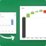
Excel Visualization: A Guide to Clear Data Presentation for Beginners

I once struggled with dull data tables.

Numbers clustered in rows and columns become a blur. But with Excel visualization , you can empower your audience to make informed decisions based on the data presented. Excel charts and graphs replace chaos, revealing patterns and trends.

Convey ideas efficiently with the right visual. It’s not just about creating a chart; it’s about making data understandable and engaging.

In this article, I’ll guide you step-by-step on transforming your Excel data into insightful visuals.

Let’s get started!

Table of Contents

Understanding the Basics of Excel Visualization

Excel provides various visualization options, whether 2D or 3D versions, standard, stacked, or 100% stacked options. It’s all about finding the right fit that best represents your data and message.

The Excel Charting Interface

Let’s start with creating a chart in Excel.

When you click on the Insert tab in Excel, you’ll see various chart types that you can use to visualize your data.

The Excel charting interface provides a wide range of options, from line and area charts to bar and column charts. When you click on a chart, the ‘ Chart Tools ’ contextual tab provides additional features for customizing your charts.

Types of Data for Visualization

Excel visualization data can be broadly categorized into numerical, categorical, and time-series data.

• Numerical data includes values that can be measured, such as sales figures or temperature readings.
• Categorical data includes information such as names, labels, or groups.
• Time-series data involves values measured over time, such as stock prices or website traffic.

Excel offers different chart types depending on your data type.

Selecting the Right Chart Type

Selecting the right chart type is half the battle for effective data visualization in Excel.

Pie charts are best for part-to-whole comparisons. Use line charts for time series or trends. Bar or column charts are the most suitable for categorical comparisons.

However, consider more advanced chart types for more complex data sets.

Scatter plots are excellent for correlation analysis , while histograms and box plots are ideal for distribution analysis of quantitative data.

It’s all about understanding your data and determining the best way to display it.

Steps for Visualizing Data in Excel – Creating Basic Charts

Creating basic charts in Excel is a fundamental skill for anyone looking to present data in a visual format.

Excel offers a variety of chart types, each with unique properties and use cases. The key to successful chart creation in Excel is understanding these different chart types and knowing how to present your data most effectively with them.

Organizing Your Data

Before you dive into creating Excel charts, it is crucial to organize your data correctly . 

Well-organized data will make the charting process easier and the resulting charts more meaningful. Ensure your data is clean, error-free, and arranged clearly and logically.

This will make it easier to select the data for your charts and create visuals that effectively communicate your data analysis results.

Pie and Donut Chart

Pie charts are popular for showing the proportion of different categories within a whole. While visually appealing, they are often misused and can lead to misleading interpretations.

Generally, they are most effective when comparing a few categories representing parts of a whole.

On the other hand, donut charts are a variation of pie charts with a hole in the middle (as the name implies!). Like pie charts, they can display multiple data series, but they should be used sparingly.

To create a pie chart in Excel:

• Select the data you want to visualize
• From the “ Insert ” tab, choose “ Pie ” from the chart options.
• You can customize your chart by changing the colors, adding labels, and adjusting other settings in the “ Format Chart Area ” pane.

Here’s a video guide on how to create a donut chart:

Line and Area Chart

Line and area charts are handy when dealing with time-series data . These charts plot data points on a graph and connect them with a line, allowing you to see trends over time. 

Check out this video for a step-by-step guide on how to create a line chart:

One of the business essentials when working with line and area charts is customizing the axis and gridlines. This can help make your chart more readable and meaningful .

The “ Format Axis ” pane allows you to customize the axis labels, adjust the scale, and add gridlines.

Column and Bar Graph

Bar and column charts are Excel’s most commonly used chart types. They are excellent for comparing different categories of data.

While bar charts and column charts are often used interchangeably, there is a difference: A bar chart presents data horizontally , while a column chart presents data vertically . This distinction can influence how easily your audience interprets the chart.

You can also choose between a stacked or clustered bar and column chart layout.

In a stacked chart , data series are stacked on each other, while in a clustered chart , they are placed side by side.

To create a bar or column chart:

• Select the data
• Then choose either “Bar” or “Column” from the chart options in the “ Insert ” tab
• Remember to format the chart and the axis labels to make the chart easier to understand

Advanced Charting Techniques

In this section, I’ll describe how to present complex data in a visually appealing and easily understandable format. Since each dataset is unique, treat these charts as ideas for meaningfully presenting your data.

Combination Charts

This type of chart combines the features of line and column charts, allowing you to present mixed data more comprehensively.

For example, when you have a target and actual data for comparison , a combination chart can be the perfect tool for visualization.

Clicking the Chart Design tab on the ribbon allows you to change the chart type and create a customized combination chart.

This allows you to have your target values in columns and the actual values marked along the line, which provides a clearer visualization of your data.

Trendlines and Data Analysis

Another essential feature of Excel charts is the ability to add trendlines. These can be linear, polynomial, or moving average trendlines.

A trendline graphically displays trends in your data , and you can extend it beyond the actual data to predict future values.

Along with trendlines, interpreting R-squared values is also crucial in data analysis. This will help you understand the relationship between your dependent and independent variables, thus enhancing your analysis results.

Check out our detailed how-to post on adding trendlines to Excel charts .

Conditional Formatting in Charts

Conditional formatting is another advanced charting technique in Excel that can enhance your data visualization. You can also add data bars, color scales, and icon sets.

These features allow you to customize your charts based on certain conditions, making it easier for your audience to understand your data. Applying these formatting options enables you to create more engaging and visually appealing charts for your data presentation.

Creating a Tornado Chart in Excel

Tornado charts are particularly effective when comparing and contrasting different variables . A well-crafted tornado chart can help you visualize how changes in several factors can impact a specific outcome – for example, the impact of inflation on NPV and IRR results.

Here’s a video showing you how to create a tornado chart:

Designing a Funnel Chart in Excel

Funnel Charts in Excel are highly effective tools for monitoring sales processes or any other process that narrows down over time.

Here are two quick methods for designing funnel charts in Excel:

Building a Waffle Chart in Excel

Waffle charts, also known as square pie or waffle bar charts, are a great way to visualize individual data points compared to the whole data set. They are a fun and engaging way to present percentages or proportions.

Here is a simple method for creating waffle charts:

Data Visualization Tips – Enhancing Chart Aesthetics

The aesthetics of your Excel chart play a significant role in how effectively your data is communicated.

A visually appealing chart is easier to understand and engages your audience. Enhancing chart aesthetics involves working with various chart elements and features, such as colors, styles, and data labels.

Adding data labels, for instance, provides additional information on your chart, making it easier to interpret.

Besides, you can customize the chart’s colors and styles to match your presentation theme or company branding.

Check out this post for more information on good dashboard design principles .

Working with Chart Elements

Working with chart elements can significantly improve the readability and effectiveness of your data visualization.

Some key chart elements you can manipulate include titles, legends, and data labels.

• Data labels provide additional context to your data and can be customized to suit your chart
• Modify axis labels and gridlines to adjust their appearance and improve readability. Check out this video on how to add gridlines to your Excel charts:

These chart elements can enhance your aesthetic appeal and make your data easier to interpret.

Customizing Chart Colors and Styles

Spicing up your Excel charts is easier than you think.

The ‘ Chart Design ‘ tab in the Excel ribbon allows you to alter your charts’ aesthetics significantly.

Navigate to the ‘ Chart Styles ‘ section, and you’ll see various styles for your chart. 

Looking for a bit more customization? No problem! Simply click the ‘ Change Colors ‘ dropdown and choose a color scheme.

You can use Excel’s preset color schemes or create a custom color palette for brand consistency. Minor visual changes can significantly affect your chart’s overall look and feel.

3D Charts and Effects

Adding a third dimension to your charts can make them pop . But be careful.

While 3D effects can add a specific wow factor, they can also lead to misinterpretations of your data if they are not used properly.

To add 3D effects to your charts, click the ‘ Chart Styles ‘ and choose a style with 3D effects. 

Remember, though, that 3D effects should be used sparingly and only when they can enhance the understanding of the data. Overuse of these effects can lead to cluttered, confusing charts. When it comes to 3D effects, less is often more .

Advanced Excel Graphics

Beyond the basic charts, Excel offers advanced graphics capabilities to take your data presentation to the next level.

This includes using Sparklines, shapes, and icons, among other features.

Sparklines are mini-charts within individual cells, each representing a row of data. They give a quick snapshot of trends, helping you understand your data at a glance.

Excel offers line, column, and win/loss types of Sparklines that you can add with the Quick Analysis tool.

Using Shapes and Icons

Remember to appropriately format these shapes and icons to convey the right message and not distract from the data.

Portraying a Story Through Data

Excel visualization is not just about creating charts or diagrams; it’s about telling a story with your data. This is where the concept of data storytelling comes in.

It’s about using visualization tools to highlight key points and trends in your data, making it easier for your audience to understand and absorb.

It’s not unlike creating a plot in a novel where rows and columns of data are the characters, and the chart is the narrative arc. Every element should convey your story effectively and compellingly, from simple bar charts to intricate trend analysis.

Exporting and Sharing Your Visualizations

Once you’ve created your data visualization in Excel, it’s important to know how to share it! This involves exporting the visual representation of data in a format that others can easily access.

Whether you’re sharing a simple bar graph or a complex infographic, the export method will depend on the intended use of the chart/graphic.

This process can be as simple as saving your chart as an image or embedding Excel visuals in PowerPoint presentations and documents.

Saving Charts as Images

One of the simplest ways to share visualizations is by saving them as images .

To do this, right-click the chart and select ‘Save as Picture.’ Several image formats are available, each with its uses.

For instance, JPEG is great for photographic images, while PNG is ideal for images with transparent backgrounds. However, it’s important to consider the resolution of your image. High resolution is crucial for clear, crisp images, especially if they’re intended for print.

Embedding Excel Visuals in Presentations and Documents

Embedding them in presentations and documents is another way to share your Excel visualizations.

This can be done in two ways: linking and embedding .

• Linking refers to connecting the original Excel file and the document where it’s inserted. Any changes made to the original file will automatically update in the document (assuming the link isn’t broken ).
• Embedding involves inserting a copy of the chart into the document. While this won’t update automatically, it ensures that the chart will always be available, regardless of the status of the original file.

Both methods have advantages and should be chosen based on your specific needs.

Frequently Asked Questions

What are some common mistakes for beginners to avoid in data visualization with excel.

Common mistakes include overcrowding the chart with too much data, using inappropriate chart types, neglecting to label axes or data points clearly, and choosing colors or styles that reduce readability.

What are the best practices for presenting Excel data visually to a non-technical audience?

Focus on simplicity and clarity .

Use straightforward chart types, avoid technical jargon, and highlight key takeaways. Ensure your charts are well-labeled, and use annotations or callouts to draw attention to important data points.

What are some resources to learn more about Excel visualization? 

For more tips and tricks, visit my YouTube channel . Alternatively, look at Chandoo’s training, where I learned many excellent dashboard design ideas.

Can Excel visualization help in career development?

Absolutely! Proficiency in Excel visualization is a valuable skill in many industries.

It’s especially relevant in fields like data science, finance, marketing, and others involving large amounts of data. Effectively communicating data through graphical representation can give you a significant advantage in your professional journey.

Leave a Comment Cancel reply

Save my name, email, and website in this browser for the next time I comment.

• Excel Charts Tutorial
• Excel Charts - Home

Excel Charts - Introduction

• Excel Charts - Creating Charts
• Excel Charts - Types
• Excel Charts - Column Chart
• Excel Charts - Line Chart
• Excel Charts - Pie Chart
• Excel Charts - Doughnut Chart
• Excel Charts - Bar Chart
• Excel Charts - Area Chart
• Excel Charts - Scatter (X Y) Chart
• Excel Charts - Bubble Chart
• Excel Charts - Stock Chart
• Excel Charts - Surface Chart
• Excel Charts - Radar Chart
• Excel Charts - Combo Chart
• Excel Charts - Chart Elements
• Excel Charts - Chart Styles
• Excel Charts - Chart Filters
• Excel Charts - Fine Tuning
• Excel Charts - Design Tools
• Excel Charts - Quick Formatting
• Excel Charts - Aesthetic Data Labels
• Excel Charts - Format Tools
• Excel Charts - Sparklines
• Excel Charts - PivotCharts
• Excel Charts Useful Resources
• Excel Charts - Quick Guide
• Excel Charts - Useful Resources
• Excel Charts - Discussion
• Selected Reading
• UPSC IAS Exams Notes
• Developer's Best Practices
• Questions and Answers
• Effective Resume Writing
• HR Interview Questions
• Computer Glossary

In Microsoft Excel, charts are used to make a graphical representation of any set of data. A chart is a visual representation of data, in which the data is represented by symbols such as bars in a bar chart or lines in a line chart.

Charts Group

You can find the Charts group under the INSERT tab on the Ribbon.

The Charts group on the Ribbon looks as follows −

The Charts group is formatted in such a way that −

Types of charts are displayed.

The subgroups are clubbed together.

It helps you find a chart suitable to your data with the button Recommended Charts.

Chart Tools

When you click on a chart, a new tab Chart Tools is displayed on the ribbon. There are two tabs under CHART TOOLS −

Recommended Charts

The Recommended Charts command on the Insert tab helps you to create a chart that is just right for your data.

To use Recommended charts −

Step 1 − Select the data.

Step 2 − Click Recommended Charts .

A window displaying the charts that suit your data will be displayed.

• school Campus Bookshelves
• menu_book Bookshelves
• perm_media Learning Objects
• login Login
• how_to_reg Request Instructor Account
• hub Instructor Commons
• Download Page (PDF)
• Download Full Book (PDF)
• Periodic Table
• Physics Constants
• Scientific Calculator
• Reference & Cite
• Tools expand_more
• Readability

selected template will load here

This action is not available.

2: Graphical Representations of Data

• Last updated
• Save as PDF
• Page ID 22222

In this chapter, you will study numerical and graphical ways to describe and display your data. This area of statistics is called "Descriptive Statistics." You will learn how to calculate, and even more importantly, how to interpret these measurements and graphs.

• 2.1: Introduction In this chapter, you will study numerical and graphical ways to describe and display your data. This area of statistics is called "Descriptive Statistics." You will learn how to calculate, and even more importantly, how to interpret these measurements and graphs. In this chapter, we will briefly look at stem-and-leaf plots, line graphs, and bar graphs, as well as frequency polygons, and time series graphs. Our emphasis will be on histograms and box plots.
• 2.2: Stem-and-Leaf Graphs (Stemplots), Line Graphs, and Bar Graphs A stem-and-leaf plot is a way to plot data and look at the distribution, where all data values within a class are visible. The advantage in a stem-and-leaf plot is that all values are listed, unlike a histogram, which gives classes of data values. A line graph is often used to represent a set of data values in which a quantity varies with time. These graphs are useful for finding trends.  A bar graph is a chart that uses either horizontal or vertical bars to show comparisons among categories.
• 2.3: Histograms, Frequency Polygons, and Time Series Graphs A histogram is a graphic version of a frequency distribution. The graph consists of bars of equal width drawn adjacent to each other. The horizontal scale represents classes of quantitative data values and the vertical scale represents frequencies. The heights of the bars correspond to frequency values. Histograms are typically used for large, continuous, quantitative data sets. A frequency polygon can also be used when graphing large data sets with data points that repeat.
• 2.4: Using Excel to Create Graphs Using technology to create graphs will make the graphs faster to create, more precise, and give the ability to use larger amounts of data. This section focuses on using Excel to create graphs.
• 2.5: Graphs that Deceive It's common to see graphs displayed in a misleading manner in social media and other instances. This could be done purposefully to make a point, or it could be accidental. Either way, it's important to recognize these instances to ensure you are not misled.
• 2.E: Graphical Representations of Data (Exercises) These are homework exercises to accompany the Textmap created for "Introductory Statistics" by OpenStax.

Contributors and Attributions

Barbara Illowsky and Susan Dean (De Anza College) with many other contributing authors. Content produced by OpenStax College is licensed under a Creative Commons Attribution License 4.0 license. Download for free at http://cnx.org/contents/[email protected] .

30 day money back guarantee

11 Best Excel Graph Creators (2024) [FREE]

1. introduction.

Creating visual graphical representation of data is essential in today’s data-driven world. The ability to clearly present complex data sets can significantly enhance the communication and understanding of information. An Excel graph creator can greatly simplify the creation of these visual repsentations, offering a wide array of chart types, data manipulation tools, and customizable features to perfectly fit your specific needs.

1.1 Importance of Excel Graph Creator

Excel Graph Creators are flung into this era of data visualization and make it easier to understand and interpret data. They are vital tools that turn abstract numbers into comprehendible visuals, making data more digestible for everyone, irrespective of their level of data literacy. They add clarity to reports, presentations and analysis, making communication more effective.

1.2 Objectives of this Comparison

The following comparison is aimed at providing a clear and thorough review of the various Excel graph creators available today. By highlighting their pros and cons, this analysis will assist users in finding the right tool that fits their unique needs and requirements. Additionally, the comparison will serve as a valuable resource for those seeking to understand the functionality and usability of these tools in detail.

1.3 Fix Excel Files

You also need a professional tool to fix Excel files in case they are corrupt. DataNumen Excel Repair is a popular one:

2. Visme Online Graph Maker

Visme is a cloud-based visual content creation and collaboration platform, empowering anyone to create professional, branded content no matter their design background. With its online graph maker, you can easily create stunning charts and graphics by simply uploading your data. Offering a diverse range of pre-made templates and customizable features, Visme aims to make data visualization efficient and effective.

• Easy to use: Visme is known for its user-friendly interface, which makes graph creation a hassle-free process.
• Highly customizable: It offers a great deal of customization options for creating differentiated visuals, allowing users to adjust colors, fonts, and images as per their requirements.
• Integration capabilities: Visme can seamlessly integrate with numerous other applications and platforms, facilitating data upload and visualization.
• Cross-platform access: Being a cloud-based tool, Visme allows you to create, edit, and access your graphs from any device with internet access.
• Limitations of the free version: While a free version of Visme is available, it comes with limited features. Full access to premium features requires a paid upgrade.
• Learning curve: Despite an easy-to-use interface, initial usage might require some time to get used to its plethora of features.
• Internet dependent: As Visme is an online tool, uninterrupted internet connectivity is required to work without disruptions.

3. LiveGap Charts Excel Graph Creator

LiveGap Charts is a free online chart maker that allows you to create all types of graphs such as bar charts, line plots, histograms, radial bar charts, and more from Excel data. No setup is required, and intuitive functionality makes this tool easy to navigate for those with little or no prior experience in data visualization.

• Free of charge: Unlike many other visualization tools, LiveGap Charts offers its complete range of features at no cost.
• No registration required: LiveGap Charts allows instant use without the necessity for a registered account.
• Compatibility: LiveGap can process data input directly from Excel spreadsheets, making it highly compatible for users primarily working with Excel.
• Diverse range of chart types: The platform enables creation of a wide variety of charts, this flexibility allows users to choose the most suitable visual representation for their dataset.
• Limited customization: Compared to other tools, customization offerings are relatively limited. The aesthetic changes you can make to your graphs might not fully meet all users’ needs.
• Lacks advanced features: More intricate graphing features that are typical of some paid services might not be present in LiveGap.
• No user support or guides: LiveGap falls short when it comes to user assistance or step-by-step guides for their tools.

4. Piktochart Online Graph Maker

Piktochart is a versatile online graph maker that enables users to create interesting, customizable graphics including charts and infographics. Piktochart serves as a canvas for non-artists to create beautiful, high-quality visuals without needing a professional designer’s skills set.

• Templated designs: Piktochart provides a variety of templates, making the graph creation process quick and easy.
• User-friendly interface: Its drag-and-drop design makes the tool accessible to individuals without extensive technical know-how.
• Inbuilt icons and images: It offers an extensive library of built-in icons and images that users can incorporate in their designs to make them more engaging and appealing.
• High-quality output: Piktochart excels in producing high-resolution images, which is beneficial for presentations and printouts.
• Internet Dependent: Being an online tool, Piktochart requires a stable internet connection to function properly.
• Limited free version: While the tool hosts a free version, the access to features and options are limited unless upgraded to the paid version.
• Complex graphics: Piktochart is not well-suited for creating complex graphs and diagrams, where deep customization and advanced features are needed.

5. Fotor Online Graph Maker

Fotor is an all-in-one online graphic design and image editing tool, which includes features for creating custom graphs. It’s also known for its photo editing capabilities, with Photoshop-like features included in its suite. Fotor is suitable for individuals and small businesses searching for a multi-purpose design tool that can create graphics and edit pictures.

• Fotor for graphics and photos: Fotor is not exclusively a graph maker; rather, it’s a full-featured image editing tool, making it a one-stop shop for all graphic needs.
• Templates: Fotor provides an array of template options for charts and infographics, simplifying the design process for users.
• User-friendly interface: The tool is straightforward to navigate; even newcomers can easily understand how to use the features.
• Advanced image editing features: Fotor’s image editor is comparable to Photoshop in its capabilities, providing many options for image manipulations.
• Preserves quality exclusively for pro users: High-resolution exports and quality preservations are available exclusively to paid users.
• Ad-filled free version: The free version of the tool is filled with ads which hinder the user experience.
• Not specifically designed for graphs: Being primarily an image editing tool, although it includes graph maker features, you might not find some in-depth charting functionalities offered by dedicated graph-making software.

6. Venngage Free Online Graph Maker

Venngage is a free online graph maker that allows users to design and publish infographics, charts, reports, and more. Venngage specializes in transforming dry, complex data into visually stunning, easy-to-understand infographics. It provides a variety of templates to help users get started quickly, and offers quite a wide range of customization options for charts.

• Intuitive user interface: Venngage offers a user-friendly environment suitable for both novices and professionals, making graph creation a breeze.
• Wide selection of templates: The tool provides a myriad of ready-made templates, making it quick and straightforward to create visually appealing graphs.
• Extensive library of icons: Venngage boasts a library of thousands of icons that can be easily added to graphs, enhancing their visual appeal.
• Inbuilt guide: It’s accompanied by helpful tips and guides that are beneficial, particularly for those new to data visualization.
• Limitations in the free version: All features of Venngage are not available in the free version, certain advanced design features require a paid upgrade.
• Slow performance: Users have reported the tool can be somewhat slow, especially when handling larger data sets.
• Exporting issues: There have been reports of some issues or restrictions with exporting the finished graphs, which can affect the overall user experience.

7. ChartGo Online Chart Maker

ChartGo is an intuitive online chart making tool that is well-suited for quick and simple chart generation. It offers a streamlined interface, and creates charts in a few easy steps by simply inputting your data. Its simplicity and ease-of-use make ChartGo a viable choice for users seeking a straightforward solution for effective chart creation.

• Simple interface: ChartGo has an uncomplicated and intuitive interface, making it ideal for those looking for quick chart creation.
• No registration needed: The ability to create charts without setting up an account allows instant use of the service.
• Various chart types: Despite the simplicity, ChartGo supports the creation of several types of charts, including line, bar, and pie charts.
• Image format output: Charts can be exported as image files for easy inclusion in reports and presentations.
• Limited customization: Compared to other tools, customization options are relatively limited, impeding the creative flexibility.
• Basic Feature Set: The feature set is limited, mainly focusing on basic chart creation, and might not suffice for more complex graphs.
• No data storage: ChartGo does not store data or chart configurations, making it difficult to revise and update charts.

8. Origin and OriginPro

Origin and OriginPro, developed by OriginLab, provide a comprehensive solution for creating customized graphs and performing advanced data analysis. They are widely accepted tools in the scientific community due to their extensive functionality and precision, making them suitable for both data exploration and presentation.

• Advanced graphing capabilities: Origin allows users to create highly advanced, detailed, and custom graphs, beyond the capabilities of standard graph software.
• Data Analysis: Apart from graphing, OriginPro also offers a variety of data analysis tools which are beneficial for researchers and analysts.
• Batch plotting: You can generate same-style graphs from multiple data sets, saving time when dealing with high-volume data.
• Compatibility: Origin software has impressive compatibility with various data formats and includes integration with LabTalk, Python and C, offering greater flexibility.
• High learning curve: Due to its advanced functionality, Origin software has a steep learning curve compared to more simplistic graphing tools.
• Cost: Instead of a monthly licensing fee, OriginLab charges a hefty one-time payment for their software, which might be expensive for some users.
• Complex interface: The interface can seem cluttered and overwhelming to new users due to its abundance of tools and features.

9. SmartDraw Excel Graph Creator

SmartDraw is a powerful online chart maker that specializes in diagramming and visualization. Its advanced features allow you to create all types of professional-quality graphs from directly within your Excel data, making it ideal for users who are looking for robust graph creation features enhanced by the power of Excel.

• Integration with Excel and other apps: SmartDraw is compatible with Excel for streamlined data importing and it also integrates with popular tools like Google Docs, MS Office, and others.
• Large selection of templates: The tool features an extensive library of templates that cover a wide range of chart types and styles.
• Collaborative functions: SmartDraw supports multiple collaborative features such as comments and sharing, perfect for team-based projects.
• Automatic formatting: Charts and diagrams can be automatically formatted, saving users valuable time.
• Cost: The tool is not free, which might deter some users. The different functions and advanced tools come at an expense.
• Complex Tool: Users might experience a learning curve due to its extensive features and functionalities.
• Performance issue: Users have reported performance issues at times with the software taking extra time to load and respond.

DPlot is a software designed for scientists, engineers, and students for data visualization and manipulation. DPlot’s Excel add-in allows users to create a wide variety of different graph types from Excel data. Including combinations of 2D and 3D plot types, DPlot provides an extensive framework for data visualization.

• Extensive Plotting Capabilities: DPlot offer users a range of plotting options, including 2D, 3D, polar, contour and surface plots.
• Data Manipulation Functions: The tool provides a variety of data manipulation functions inclusive of FFT, filtering, and smoothing features.
• Accurate Data Representation: DPlot is recognized for its ability to handle large data sets, providing accurate and detailed graphical representation.
• Excel Integration: The software has an Excel add-in making the process of creating graphs from Excel data more effortless and efficient.
• Outdated Interface: The interface of DPlot can seem outdated to some users, potentially making navigation harder than modern interfaces.
• Cost: Unlike some other graphing tools, DPlot is not free and requires a purchase.
• Learning Curve: DPlot’s abundance of features may pose a steep learning curve for new users.

11. GraphMaker Excel Graph Creator

GraphMaker is a powerful and intelligent tool that simplifies the process of creating graphs from Excel data. Designed with artificial intelligence, this tool automatically generates charts based on your dataset. Its aim is to help users turn raw data into insightful and visually appealing graphs, and quickly identify trends and patterns in their data.

• AI-Powered: GraphMaker utilizes artificial intelligence to interpret data and create suitable graphs, easing the graph generation process.
• User-friendly interface: The easy-to-use interface is designed for both experienced and inexperienced users.
• Automation: It automates the process of reading data fields, interpreting them, and creating an engaging visual summary.
• Insightful data visualization: The created graphs are not only visually appealing, but also highly insightful, helping users identify patterns and trends in their data.
• Limited customisation options: Although the tool automatically creates graphs, users have reported fewer options for customizing graphs compared to other tools.
• Dependency on AI: Since the tool is AI-based, there can be instances when AI makes decisions about the type of graph that may not align with users’ requirements.
• Connectivity requirements: As it’s an online tool, users need a stable internet connection to use GraphMaker.

12. Moqups Free Online Graph Maker

Moqups is a versatile online tool famous for its functionality in creating mockups, diagrams, and prototypes. Alongside its staple features, it also includes a graph maker allowing you to produce compelling visual representations of data. The tool’s unique feature is its seamless transition from ideation phase to implementation phase all within the same workspace.

• Multifunctional: Apart from graph creation, Moqups can be also used for making wireframes, diagrams, and mockups.
• Interactive Canvas: It offers an expansive, unobstructed canvas allowing great flexibility for placing objects and creating designs.
• Team Collaboration: Moqups features a robust set of collaboration tools, making it easy to work with teams.
• Intuitive UI: The user-friendly interface of the application ensures a smooth user experience.
• Limited Free Version: The free version of Moqups comes with restricted features and users must upgrade to access all functionalities.
• Internet Dependent: As it’s a web-based application, continuous internet connectivity is required for uninterrupted usage.
• Not specifically built for graphing: While it does offer graph-making capabilities, the primary focus of Moqups is prototyping and mockup design, possibly limiting its graph-making potential.

13. Summary

13.1 overall comparison table, 13.2 recommended tool based on various needs.

For beginners: If you’re a beginner looking for an easy-to-use tool, then Visme or Piktochart would be ideal, as they offer a user-friendly interface and a variety of ready-made templates.

For scientists and researchers: For those in search of more analytical functionalities and advanced features, software like Origin and OriginPro or DPlot would be your best bet.

For budget-conscious users: Users on a budget can utilize free tools like LiveGap Charts, ChartGo, or the free versions of many of the mentioned tools.

For AI-driven automation: If you’re looking for automation in graph creation, GraphMaker can be a perfect choice with its AI-powered features.

For team collaboration: For those in team settings, the collaboration feature of Moqups would be of great use.

14. Conclusion

14.1 final thoughts and takeaways for choosing an excel graph creator.

Choosing the right Excel graph creator is a decision that should be based on your unique needs and requirements. Bear in mind specific criteria like the ease-of-use, the variety of features, the customer support, and the pricing model. If you’re a beginner, consider tools with an intuitive interface and ready-made templates. If you’re a professional or researcher, opt for tools offering advanced features and intricate plotting capabilities. Budget-conscious users might want to utilize free tools while teams might favor tools with collaborative features.

Every tool mentioned in this comparison has its distinct strengths, addressing different needs and preferences. You might need to try out several of these before settling on the one that aligns perfectly with your needs. In the world of digital data, having the right tool to effectively visualize your data in a meaningful and understandable way is of utmost importance. Therefore, it is important to take an informed decision when choosing the most suitable Excel graph creator for your needs.

Author Introduction:

Vera Chen is a data recovery expert in DataNumen, which provides a wide range of products, including a powerful tool to repair DWG files.

Leave a Reply Cancel reply

Your email address will not be published. Required fields are marked *